
The Poisson Distribution
1. Introduction
The Poisson distribution is the workhorse for count data — the number of times something happens in a fixed interval of time, space, or volume. Named after French mathematician Siméon Denis Poisson (1837), it appears everywhere: call-centre arrivals, radioactive decay counts, hospital admissions, insurance claims, defects in manufactured goods, and species counts in ecology plots.
Its appeal is simplicity: the entire distribution is described by a single parameter, \(\lambda\), which is simultaneously the mean and the variance.
2. Mathematical Definition
2.1 Probability Mass Function (PMF)
The probability of observing exactly \(k\) events in an interval is:
\[P(X = k) = \frac{\lambda^k e^{-\lambda}}{k!}, \quad k = 0, 1, 2, \ldots\]
where \(\lambda > 0\) is the expected rate of events per interval.
2.2 Cumulative Distribution Function (CDF)
\[F(k; \lambda) = P(X \leq k) = e^{-\lambda} \sum_{j=0}^{k} \frac{\lambda^j}{j!}\]
2.3 Key Moments
| Statistic | Value |
|---|---|
| Mean | \(\lambda\) |
| Variance | \(\lambda\) |
| Skewness | \(1 / \sqrt{\lambda}\) |
| Kurtosis | \(1 / \lambda\) |
The mean equals the variance — this is the single most important diagnostic property of the Poisson distribution.
3. Visualising the Effect of \(\lambda\)
library(ggplot2)
library(dplyr)
library(tidyr)

x_grid   <- 0:30
lam_vals <- c(1, 3, 7, 15)

pmf_df <- lapply(lam_vals, function(l) {
  data.frame(k = x_grid, prob = dpois(x_grid, l), lambda = paste0("λ = ", l))
}) |> bind_rows()

ggplot(pmf_df, aes(x = k, y = prob)) +
  geom_segment(aes(xend = k, yend = 0), color = "#4E9AF1", linewidth = 0.9) +
  geom_point(color = "#4E9AF1", size = 2) +
  facet_wrap(~ lambda, scales = "free") +
  labs(
    title = "Poisson PMF for Selected λ Values",
    x     = "Count k",
    y     = "P(X = k)"
  ) +
  theme_minimal(base_size = 13)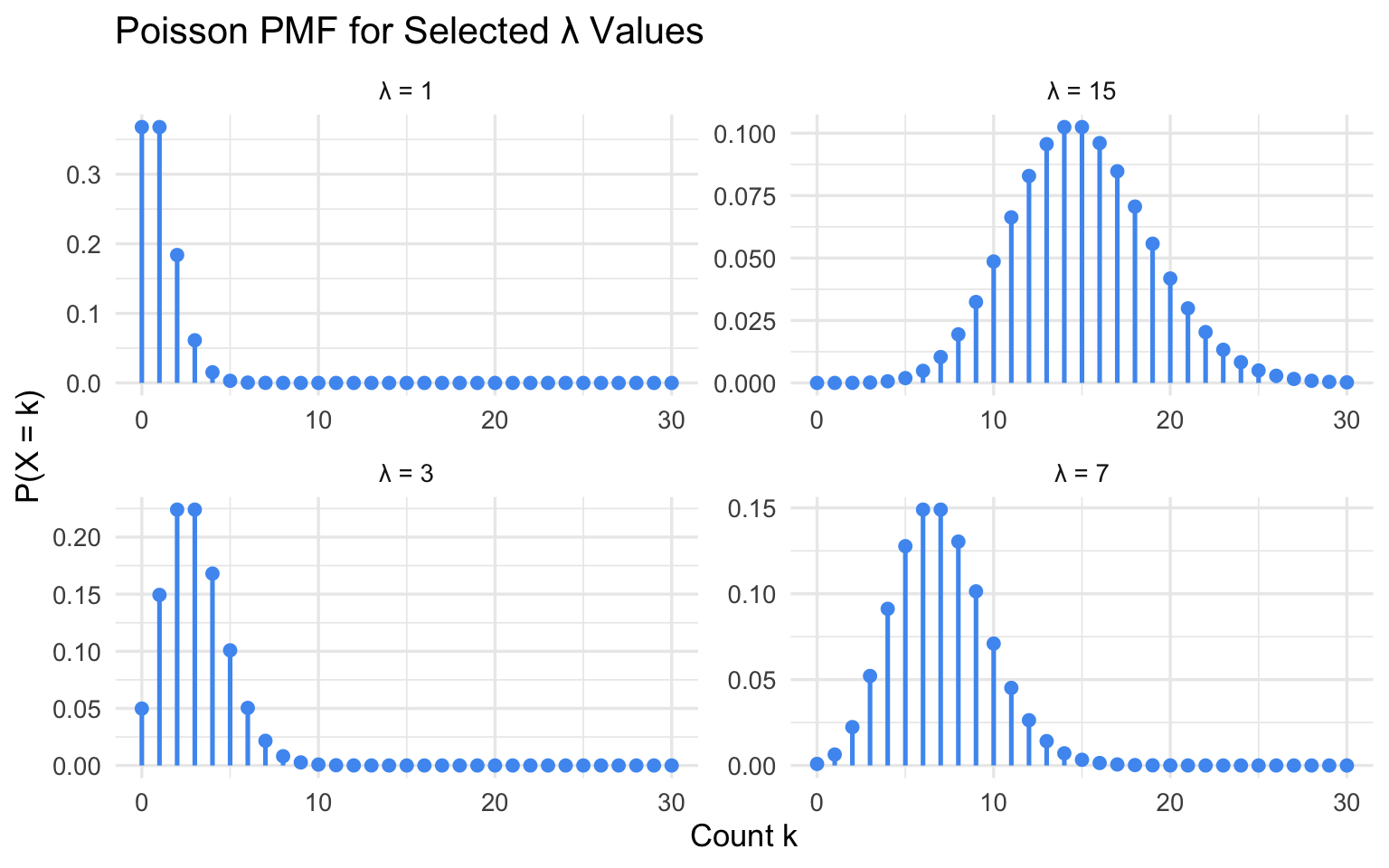
As \(\lambda\) increases the distribution shifts right, spreads out, and becomes increasingly symmetric — eventually approximating a Normal distribution.
4. R Functions
R provides four standard functions for the Poisson distribution:
lambda <- 5

# P(X = 3): probability of exactly 3 events
cat("P(X = 3):            ", round(dpois(3, lambda), 5), "\n")
## P(X = 3): 0.14037# P(X <= 3): cumulative probability
cat("P(X <= 3): ", round(ppois(3, lambda), 5), "\n")## P(X <= 3): 0.26503# P(X > 3): upper tail (lower.tail = FALSE avoids cancellation)
cat("P(X > 3): ", round(ppois(3, lambda, lower.tail = FALSE), 5), "\n")## P(X > 3): 0.73497# qpois: smallest k such that P(X <= k) >= 0.90
cat("90th percentile: ", qpois(0.90, lambda), "\n")## 90th percentile: 8# rpois: random samples
set.seed(42)
samples <- rpois(n = 1000, lambda = lambda)
cat("Sample mean: ", round(mean(samples), 4), "\n")## Sample mean: 4.914cat("Sample variance: ", round(var(samples), 4), "\n")## Sample variance: 4.8975cat("Var / Mean ratio: ", round(var(samples) / mean(samples), 4),
" (should be ≈ 1)\n")## Var / Mean ratio: 0.9966 (should be ≈ 1)5. When to Use the Poisson Distribution
Use the Poisson distribution when all five of the following conditions hold:
| Condition | Description |
|---|---|
| Count data | You are counting discrete occurrences, not measuring a continuous quantity |
| Fixed interval | Events are counted over a fixed unit of time, space, or volume |
| Independence | One event does not make another more or less likely |
| Constant rate | The average rate \(\lambda\) does not vary across intervals |
| No upper bound | There is no theoretical maximum number of events |
And as a data-driven check: sample mean ≈ sample variance.
Classic examples
scenarios <- data.frame(
  Scenario              = c("Hospital ED arrivals / hour",
                            "Typos per page in a manuscript",
                            "Radioactive decay events / second",
                            "Insurance claims / policy / year",
                            "Manufacturing defects / unit",
                            "Bacteria colonies per agar plate"),
  `Fixed interval`      = c("1 hour", "1 page", "1 second",
                             "1 year", "1 unit", "1 plate"),
  `Typical λ`           = c("12", "0.4", "0.001", "0.05", "1.5", "8")
)
knitr::kable(scenarios, align = "lcc")| Scenario | Fixed.interval | Typical.λ |
|---|---|---|
| Hospital ED arrivals / hour | 1 hour | 12 |
| Typos per page in a manuscript | 1 page | 0.4 |
| Radioactive decay events / second | 1 second | 0.001 |
| Insurance claims / policy / year | 1 year | 0.05 |
| Manufacturing defects / unit | 1 unit | 1.5 |
| Bacteria colonies per agar plate | 1 plate | 8 |
6. When NOT to Use the Poisson Distribution
6.1 Overdispersion — Variance > Mean
The most common violation. Real-world count data often show overdispersion: the variance exceeds the mean because events cluster or because individuals differ in their underlying risk. The Poisson model then underestimates variability, producing falsely narrow confidence intervals and inflated test statistics.
set.seed(42)

# Ideal Poisson data
pois_data <- rpois(500, lambda = 5)

# Overdispersed data: Negative Binomial with same mean but extra variation
od_data <- rnbinom(500, mu = 5, size = 0.8)

results <- data.frame(
  Dataset   = c("Poisson(λ=5)", "Overdispersed (NB)"),
  Mean      = c(mean(pois_data), mean(od_data)),
  Variance  = c(var(pois_data),  var(od_data)),
  `Var/Mean` = c(var(pois_data) / mean(pois_data),
                 var(od_data)   / mean(od_data))
)
knitr::kable(results, digits = 2,
col.names = c("Dataset", "Mean", "Variance", "Var / Mean"))| Dataset | Mean | Variance | Var / Mean |
|---|---|---|---|
| Poisson(λ=5) | 4.92 | 4.96 | 1.01 |
| Overdispersed (NB) | 4.95 | 34.27 | 6.93 |
A Var/Mean ratio well above 1 is a red flag for overdispersion. Values of 2–10 are common in ecological and healthcare count data.
k_range    <- 0:max(od_data)
obs_counts <- as.numeric(table(factor(od_data, levels = k_range)))
exp_counts <- dpois(k_range, mean(od_data)) * length(od_data)

bar_df <- data.frame(
  k    = rep(k_range, 2),
  freq = c(obs_counts, exp_counts),
  Type = rep(c("Observed", "Poisson expected"), each = length(k_range))
)

ggplot(bar_df, aes(x = k, y = freq, fill = Type)) +
  geom_col(position = "dodge", width = 0.7) +
  scale_fill_manual(values = c("Observed" = "#4E9AF1", "Poisson expected" = "#E63946")) +
  coord_cartesian(xlim = c(0, 25)) +
  labs(
    title    = "Overdispersed Count Data vs Poisson Expectation",
    subtitle = "Poisson underestimates high counts and the zero count",
    x        = "Count k",
    y        = "Frequency",
    fill     = NULL
  ) +
  theme_minimal(base_size = 13) +
  theme(legend.position = "top")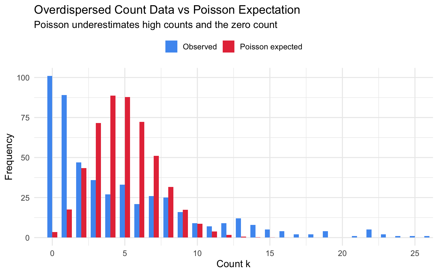
6.2 Zero-Inflation — More Zeros Than Expected
Some processes generate excess structural zeros on top of the Poisson zeros: e.g., non-smokers (structural zero) vs. smokers who happened to smoke zero cigarettes this week (Poisson zero). Forcing a Poisson fit misses the spike at zero entirely.
set.seed(42)
lambda3 <- 4
n       <- 500

# 35% structural zeros + Poisson(4) for the rest
structural_zero <- rbinom(n, 1, 0.35)
zi_counts       <- ifelse(structural_zero == 1, 0, rpois(n, lambda3))

cat("Expected zeros under Poisson(4): ", round(dpois(0, lambda3) * 100, 1), "%\n")
## Expected zeros under Poisson(4): 1.8 %cat("Observed zeros in ZIP data: ", round(mean(zi_counts == 0) * 100, 1), "%\n")## Observed zeros in ZIP data: 35.4 %k_range_zi <- 0:max(zi_counts)
obs_prop_zi <- as.numeric(table(factor(zi_counts, levels = k_range_zi))) / n
pois_prop_zi <- dpois(k_range_zi, lambda3)
zi_df <- data.frame(
k = rep(k_range_zi, 2),
prob = c(obs_prop_zi, pois_prop_zi),
Type = rep(c("Observed (ZIP)", "Poisson(4)"), each = length(k_range_zi))
)
ggplot(zi_df, aes(x = k, y = prob, fill = Type)) +
geom_col(position = "dodge", width = 0.7) +
scale_fill_manual(values = c("Observed (ZIP)" = "#4E9AF1", "Poisson(4)" = "#E63946")) +
labs(
title = "Zero-Inflated Data vs Poisson Expectation",
subtitle = "35% structural zeros — Poisson cannot account for the spike at zero",
x = "Count k",
y = "Proportion",
fill = NULL
) +
theme_minimal(base_size = 13) +
theme(legend.position = "top")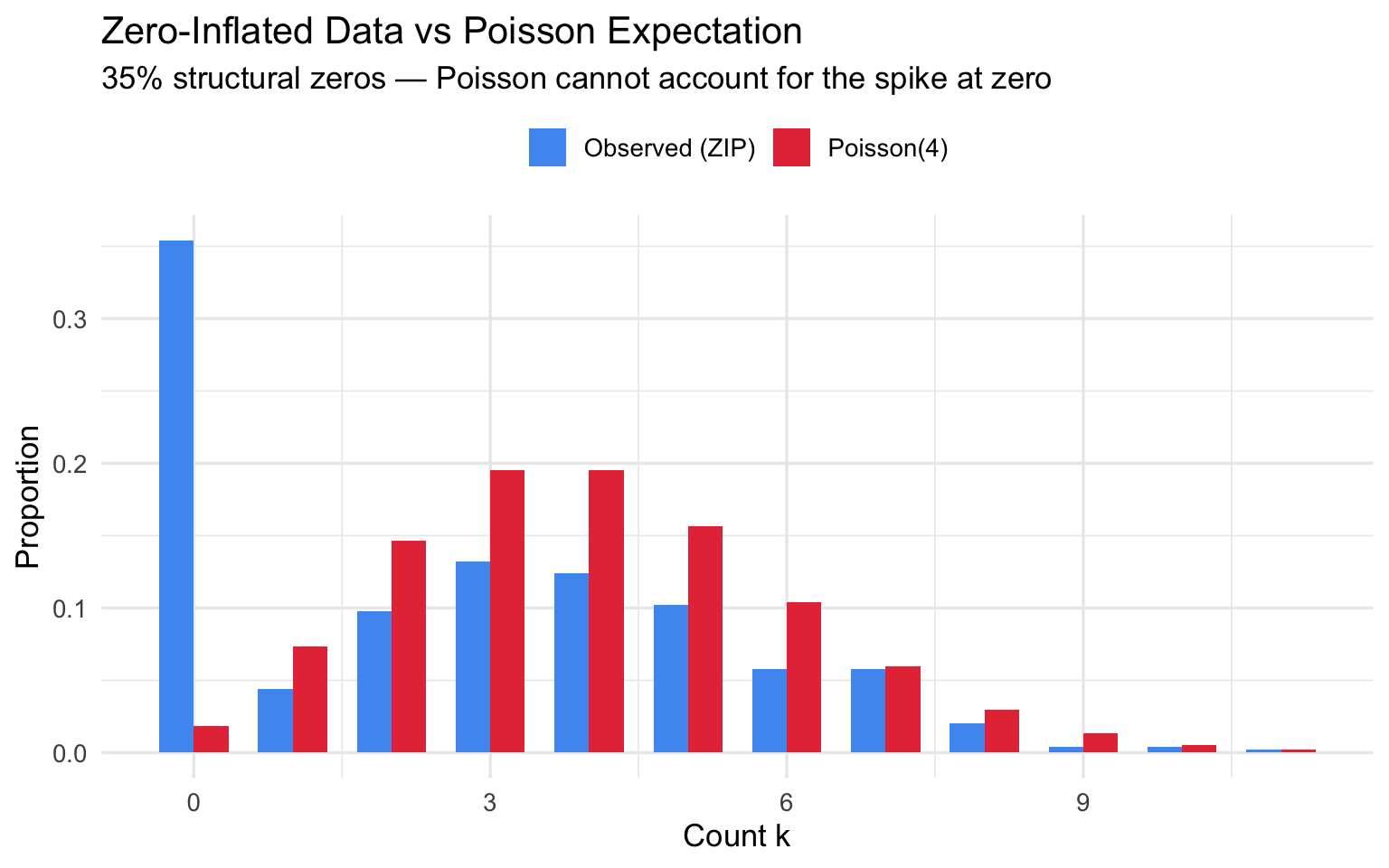
6.3 Non-Constant Rate or Non-Independence
- Contagion / clustering: one event triggers others (infectious disease, financial contagion). Events are not independent.
- Heterogeneous exposure: individuals have different underlying risk. Model with covariates in a Poisson GLM, or switch to a mixture distribution.
- Time-varying rate: arrivals at an ER peak at noon, not at 3 am. Include time as a covariate or use an inhomogeneous Poisson process.
6.4 Bounded Counts — Use Binomial Instead
If there is a fixed number of trials \(n\) and you are counting successes, the Binomial is the correct model. Poisson approximates Binomial only when \(n\) is large and \(p\) is small.
| Situation | Correct model |
|---|---|
| \(k\) successes in \(n\) fixed trials | Binomial |
| \(k\) events in a fixed interval, no upper bound | Poisson |
| \(k\) events, Var >> Mean | Negative Binomial |
| \(k\) events, excess zeros | Zero-Inflated Poisson |
7. Diagnosing: Is Poisson Appropriate?
7.1 Mean–Variance Ratio
Compute the index of dispersion \(I = s^2 / \bar{x}\):
- \(I \approx 1\) → Poisson consistent
- \(I \gg 1\) → overdispersion → consider Negative Binomial
- \(I \ll 1\) → underdispersion (rare) → consider Conway–Maxwell–Poisson
7.2 GLM Residual Deviance
Fit a Poisson GLM and check whether residual deviance ≈ degrees of freedom:
pois_glm   <- glm(od_data ~ 1, family = poisson)
disp_ratio <- pois_glm$deviance / pois_glm$df.residual

cat("Residual deviance:       ", round(pois_glm$deviance, 1), "\n")
## Residual deviance: 3019cat("Degrees of freedom: ", pois_glm$df.residual, "\n")## Degrees of freedom: 499cat("Deviance / df ratio: ", round(disp_ratio, 2), "\n")## Deviance / df ratio: 6.05cat("(Well-fitted Poisson → ratio ≈ 1)\n")## (Well-fitted Poisson → ratio ≈ 1)7.3 Formal Dispersion Test
Under Poisson, \((n-1)s^2/\bar{x} \sim \chi^2_{n-1}\):
dispersion_test <- function(x) {
  n     <- length(x)
  stat  <- (n - 1) * var(x) / mean(x)
  p_val <- pchisq(stat, df = n - 1, lower.tail = FALSE)
  cat(sprintf("  Stat: %.1f  |  df: %d  |  p-value: %.4f\n", stat, n - 1, p_val))
}

cat("Poisson data:\n");  dispersion_test(pois_data)
## Poisson data:## Stat: 503.0 | df: 499 | p-value: 0.4417cat("Overdispersed:\n"); dispersion_test(od_data)## Overdispersed:## Stat: 3456.1 | df: 499 | p-value: 0.00008. Alternatives and When to Use Them
8.1 Negative Binomial — Overdispersion
The Negative Binomial adds a dispersion parameter \(\theta\) (size). As \(\theta \to \infty\) it converges to Poisson. Use it whenever the Var/Mean ratio is substantially above 1.
\[P(X = k) = \binom{k + \theta - 1}{k} \left(\frac{\theta}{\theta + \mu}\right)^\theta \left(\frac{\mu}{\theta + \mu}\right)^k\]
library(MASS)

pois_fit <- glm(od_data ~ 1, family = poisson)
nb_fit   <- glm.nb(od_data ~ 1)

cat("Poisson AIC:       ", round(AIC(pois_fit), 1), "\n")
## Poisson AIC: 4332.2cat("Neg. Binomial AIC: ", round(AIC(nb_fit), 1), "\n\n")## Neg. Binomial AIC: 2688.3theta <- nb_fit$theta
mu_nb <- exp(coef(nb_fit)[[1]])
cat("NB estimated μ: ", round(mu_nb, 3), "\n")## NB estimated μ: 4.948cat("NB estimated θ: ", round(theta, 3), " (small θ = strong overdispersion)\n")## NB estimated θ: 0.787 (small θ = strong overdispersion)k_grid <- 0:30
model_df <- bind_rows(
data.frame(k = k_grid,
prob = dpois(k_grid, mean(od_data)),
Model = "Poisson"),
data.frame(k = k_grid,
prob = dnbinom(k_grid, mu = mu_nb, size = theta),
Model = "Neg. Binomial")
)
obs_prop <- as.numeric(table(factor(od_data, levels = k_grid))) / length(od_data)
ggplot() +
geom_col(data = data.frame(k = k_grid, prob = obs_prop),
aes(x = k, y = prob), fill = "gray80", color = "white") +
geom_line(data = model_df,
aes(x = k, y = prob, color = Model), linewidth = 1.3) +
scale_color_manual(values = c("Poisson" = "#4E9AF1", "Neg. Binomial" = "#E63946")) +
coord_cartesian(xlim = c(0, 25)) +
labs(
title = "Poisson vs Negative Binomial: Fitting Overdispersed Data",
subtitle = "Gray bars = observed proportions",
x = "Count k",
y = "Probability",
color = NULL
) +
theme_minimal(base_size = 13) +
theme(legend.position = "top")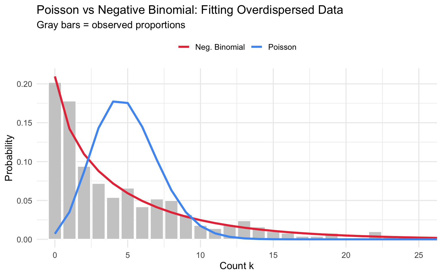
The Negative Binomial tracks the long right tail that Poisson misses entirely.
8.2 Zero-Inflated Models — Excess Zeros
Zero-Inflated Poisson (ZIP) mixes a point mass at zero with a Poisson component:
\[P(X = k) = \begin{cases} \pi + (1-\pi)e^{-\lambda} & k = 0 \\ (1-\pi)\dfrac{\lambda^k e^{-\lambda}}{k!} & k \geq 1 \end{cases}\]
where \(\pi\) is the probability of
a structural zero. The pscl package provides
zeroinfl() for both ZIP and ZINB models. Use
ZINB when you have excess zeros and
overdispersion in the non-zero counts.
8.3 Quasi-Poisson — A GLM Patch
In a GLM context, keep the Poisson log-link but relax the variance assumption to \(\text{Var}(Y) = \phi\lambda\), estimating \(\phi\) from the data. Coefficients are identical to Poisson; standard errors are inflated by \(\sqrt{\hat\phi}\).
qp_fit <- glm(od_data ~ 1, family = quasipoisson)
cat("Quasi-Poisson estimated φ:", round(summary(qp_fit)$dispersion, 3), "\n")
## Quasi-Poisson estimated φ: 6.926Quasi-Poisson is a convenient patch but does not model the mechanism behind overdispersion. Prefer Negative Binomial when interpretability matters.
8.4 Summary of Alternatives
| Problem | Recommended model |
|---|---|
| Var >> Mean (overdispersion) | Negative Binomial |
| Excess structural zeros | Zero-Inflated Poisson (ZIP) |
| Excess zeros + overdispersion | Zero-Inflated Neg. Binomial (ZINB) |
| Overdispersion, GLM context | Quasi-Poisson |
| Var < Mean (underdispersion) | Conway–Maxwell–Poisson |
| Fixed upper bound, known \(n\) | Binomial |
| Waiting time between events | Exponential |
9. Connections to Other Distributions
9.1 Poisson as the Limit of the Binomial
When \(n\) is large and \(p\) is small such that \(\lambda = np\) remains moderate, \(\text{Binomial}(n, p) \approx \text{Poisson}(\lambda)\).
n_b  <- 1000; p_b <- 0.005; lam_b <- n_b * p_b

x_range <- 0:20

approx_df <- bind_rows(
  data.frame(k = x_range, prob = dbinom(x_range, n_b, p_b),
             Distribution = paste0("Binomial(", n_b, ", ", p_b, ")")),
  data.frame(k = x_range, prob = dpois(x_range, lam_b),
             Distribution = paste0("Poisson(λ = ", lam_b, ")"))
)

ggplot(approx_df, aes(x = k, y = prob, color = Distribution)) +
  geom_line(linewidth = 1.1) +
  geom_point(size = 2) +
  scale_color_manual(values = c("#4E9AF1", "#E63946")) +
  labs(
    title    = "Poisson as a Limit of the Binomial",
    subtitle = paste0("n = ", n_b, ", p = ", p_b, "  →  λ = np = ", lam_b),
    x        = "Count k",
    y        = "P(X = k)",
    color    = NULL
  ) +
  theme_minimal(base_size = 13) +
  theme(legend.position = "top")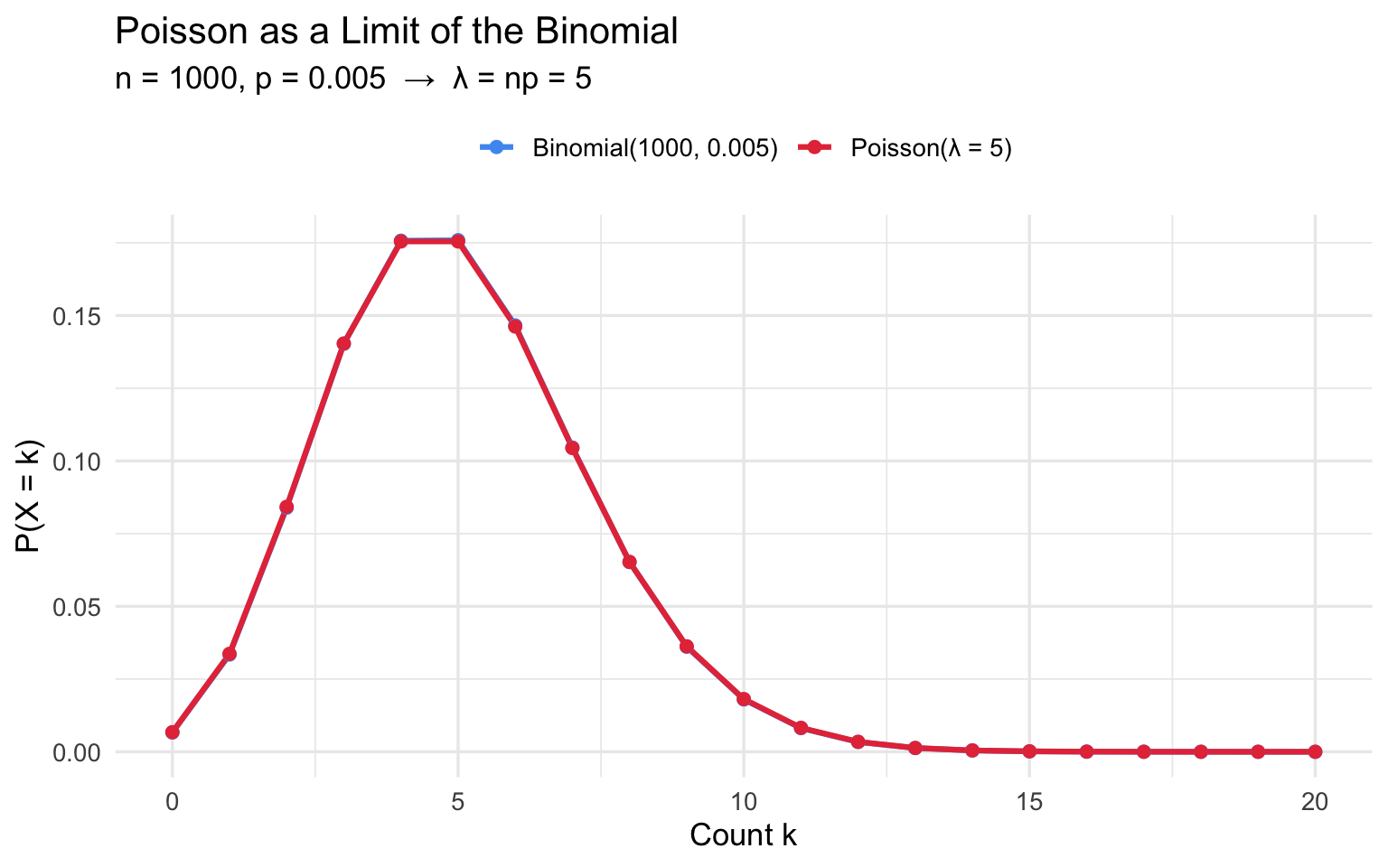
9.2 Normal Approximation for Large \(\lambda\)
For large \(\lambda\), skewness \(1/\sqrt{\lambda} \to 0\) and \(\text{Poisson}(\lambda) \approx \text{Normal}(\lambda, \lambda)\).
lam_large <- 30
x_seq     <- 0:60

norm_df <- bind_rows(
  data.frame(x = x_seq, y = dpois(x_seq, lam_large),
             Dist = paste0("Poisson(λ = ", lam_large, ")")),
  data.frame(x = x_seq, y = dnorm(x_seq, lam_large, sqrt(lam_large)),
             Dist = paste0("Normal(μ = ", lam_large, ", σ = √", lam_large, ")"))
)

ggplot(norm_df, aes(x = x, y = y, color = Dist)) +
  geom_line(linewidth = 1.2) +
  scale_color_manual(values = c("#4E9AF1", "#E63946")) +
  labs(
    title = "Normal Approximation for Large λ",
    x     = "k",
    y     = "Probability / Density",
    color = NULL
  ) +
  theme_minimal(base_size = 13) +
  theme(legend.position = "top")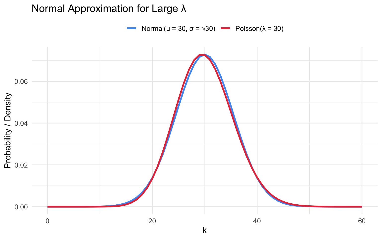
9.3 Exponential Inter-Arrival Times
If events arrive as a Poisson process with rate \(\lambda\) per unit time, the waiting time between consecutive events follows \(\text{Exponential}(1/\lambda)\). The two distributions are paired: Poisson counts events; Exponential measures the gaps between them.
10. Summary
| Topic | Key Points |
|---|---|
| Use when | Counting occurrences, fixed interval, independence, constant rate, no upper bound, Var ≈ Mean |
| Don’t use when | Var >> Mean, excess zeros, clustered events, fixed \(n\) trials |
| Diagnose with | Var/Mean ratio, deviance/df from Poisson GLM, dispersion test |
| Alternatives | Neg. Binomial (overdispersion), ZIP/ZINB (excess zeros), Quasi-Poisson (GLM patch), Binomial (bounded) |
| R functions | dpois, ppois, qpois,
rpois, glm(family=poisson),
MASS::glm.nb |
| Special connections | Limit of Binomial (large \(n\), small \(p\)); Normal approximation (large \(\lambda\)); Exponential inter-arrivals |