Color and colorspace in R

All colors

library(ggplot2)
require(colorspace)


#convenience functions
wheel <- function(col, radius = 1, ...)
  pie(rep(1, length(col)), col = col, radius = radius, ...) 

pal <- function(col, border = "light gray") {
  n <- length(col)
  plot(0, 0, type="n", xlim = c(0, 1), ylim = c(0, 1), axes = FALSE, xlab = "", ylab = "")
  rect(0:(n-1)/n, 0, 1:n/n, 1, col = col, border = border)
}
par(mfrow=c(2,2))
wheel(diverge_hcl(12))  #pal(rainbow_hcl(12))
wheel(heat_hcl(12))
wheel(rainbow_hcl(12))
wheel(sequential_hcl(12))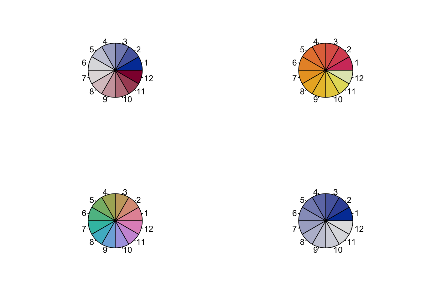

par(mfrow=c(1,1))

ColorBrewer

Represent color as a continuous variable using ColorBrewer. In ggplot2 you may use scale_brewer

require(RColorBrewer)
par(mfrow=c(2,2))
display.brewer.pal(7, "Greens")
display.brewer.pal(12, "Reds")
display.brewer.pal(7,"BrBG")
display.brewer.pal(7,"Accent")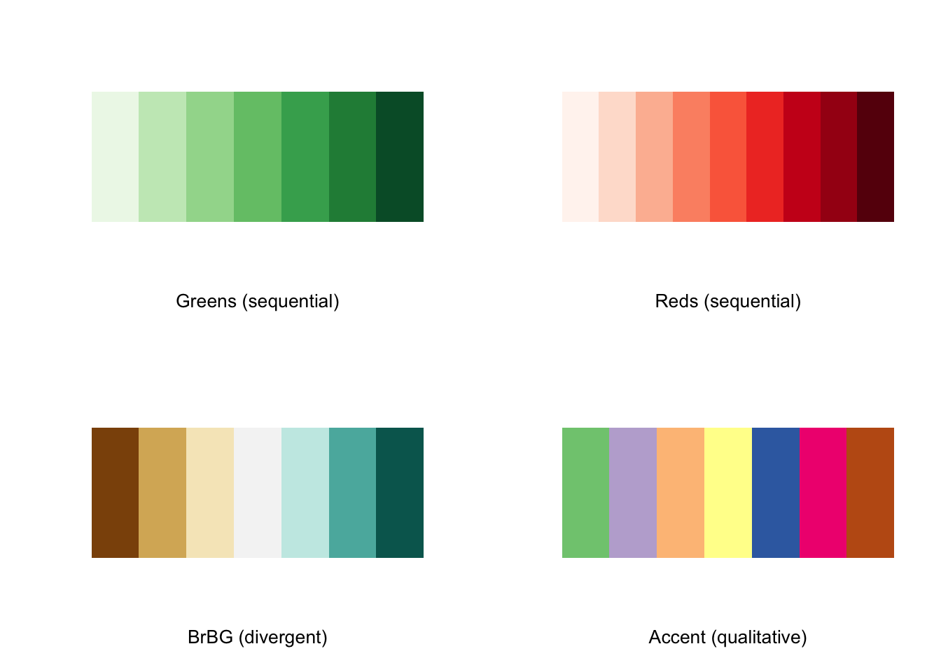

#brewer.pal.info
brewer.pal.info["Blues",]

##       maxcolors category colorblind
## Blues         9      seq       TRUE

brewer.pal.info["Blues",]$maxcolors

## [1] 9

display.brewer.all(type="qual")
display.brewer.all(type="div")
display.brewer.all(type="seq")
display.brewer.all(n=10, exact.n=FALSE)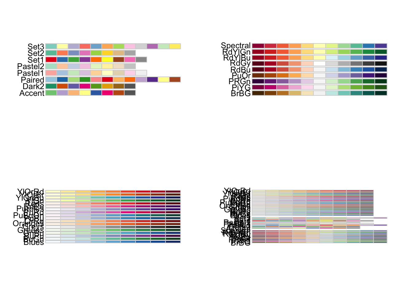

par(mfrow=c(1,1))

R Colors graphic

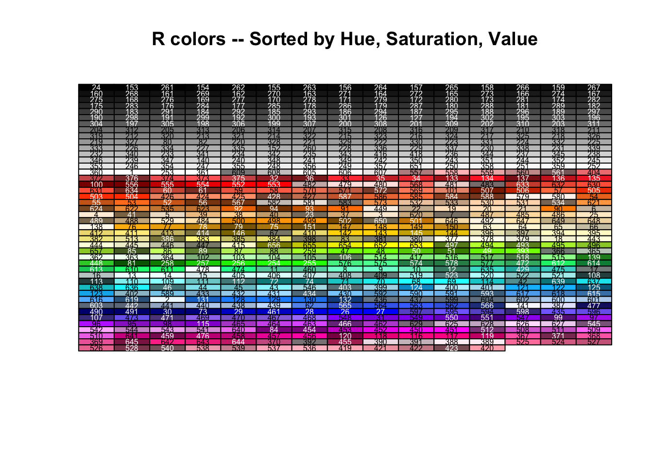
The following R code produces the “R Colors” graphic in “hue” order. The RGB values of each of the colors() was converted to hue-saturation-value (HSV) and then sorted by HSV. This approach groups colors of the same “hue” together a bit better.

# gives a good text color for a given background color name:
SetTextContrastColor <- function(color)
{
  ifelse( mean(col2rgb(color)) > 127, "black", "white")
}
# Define this array of text contrast colors that correponds to each
# member of the colors() array.
TextContrastColor <- unlist( lapply(colors(), SetTextContrastColor) )

colCount <- 15 # number per row. total 675
rowCount <- 45
RGBColors <- col2rgb(colors()[1:length(colors())])
HSVColors <- rgb2hsv( RGBColors[1,], RGBColors[2,], RGBColors[3,],
                      maxColorValue=255)
HueOrder <- order( HSVColors[1,], HSVColors[2,], HSVColors[3,] )
plot(0, type="n", ylab="", xlab="",
     axes=FALSE, ylim=c(rowCount,0), xlim=c(1,colCount))

title("R colors -- Sorted by Hue, Saturation, Value")

for (j in 0:(rowCount-1))
{
  for (i in 1:colCount)
  {
    k <- j*colCount + i
    if (k <= length(colors()))
    {
      rect(i-0.5,j-0.5, i+0.5,j+0.5, border="black", col=colors()[ HueOrder[k] ])
      text(i,j, paste(HueOrder[k]), cex=0.5, col=TextContrastColor[ HueOrder[k] ])
    }
  }
}

Luv colorspace

library(ggplot2)

x <- sRGB(t(col2rgb(colors())))
storage.mode(x@coords) <- "numeric"
y <- as(x, "LUV")
DF <- as.data.frame(y@coords)
DF$col <- colors()
g <- ggplot(DF, aes(x = U, y = V))
g + geom_point(colour = DF$col, size = I(10)) + scale_x_continuous(breaks = seq(-10000, 
    20000, 5000)) + scale_y_continuous(breaks = seq(-20000, 15000, 5000))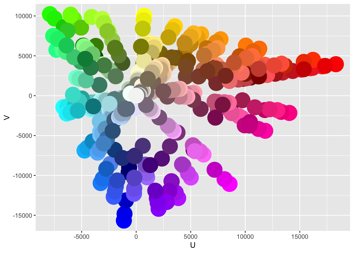

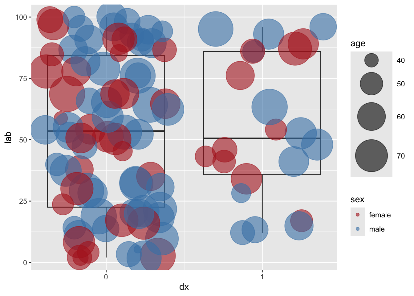
Practical examples

To manually scale the size of the points to a continuous variable, use scale_size_continuous(range = c(n, k)). Alternatively, could use scale_size_area(). With a categorical variable, the colors of the points could be set for a variable, by first defining a vector (e.g. colorSex below), then setting the aesthetics color=[variable] and finally using scale_color_manual(values=colorSex) .

library(ggplot2)
n <- 100
df <- data.frame(
  age <- rnorm (n, 60,10),
  sex <- sample(c("male", "female"), n, rep=T, prob=c(0.6, 0.4)),
  dx <- sample(c(0,1),n, rep=T, prob=c(0.75, 0.25)),
  lab <- sample (seq(1,100,1), n, rep = T)
)
colorSex <- c(male="steelblue", female="firebrick")
g <- ggplot(df, aes(group=dx, x=dx, y=lab)) +
  geom_boxplot(alpha=I(0)) + 
  geom_jitter(aes(size=age, color = sex), alpha = I(0.6)) + 
  scale_x_continuous(breaks=c(0,1)) + 
  scale_color_manual(values=colorSex)
g + scale_size_area()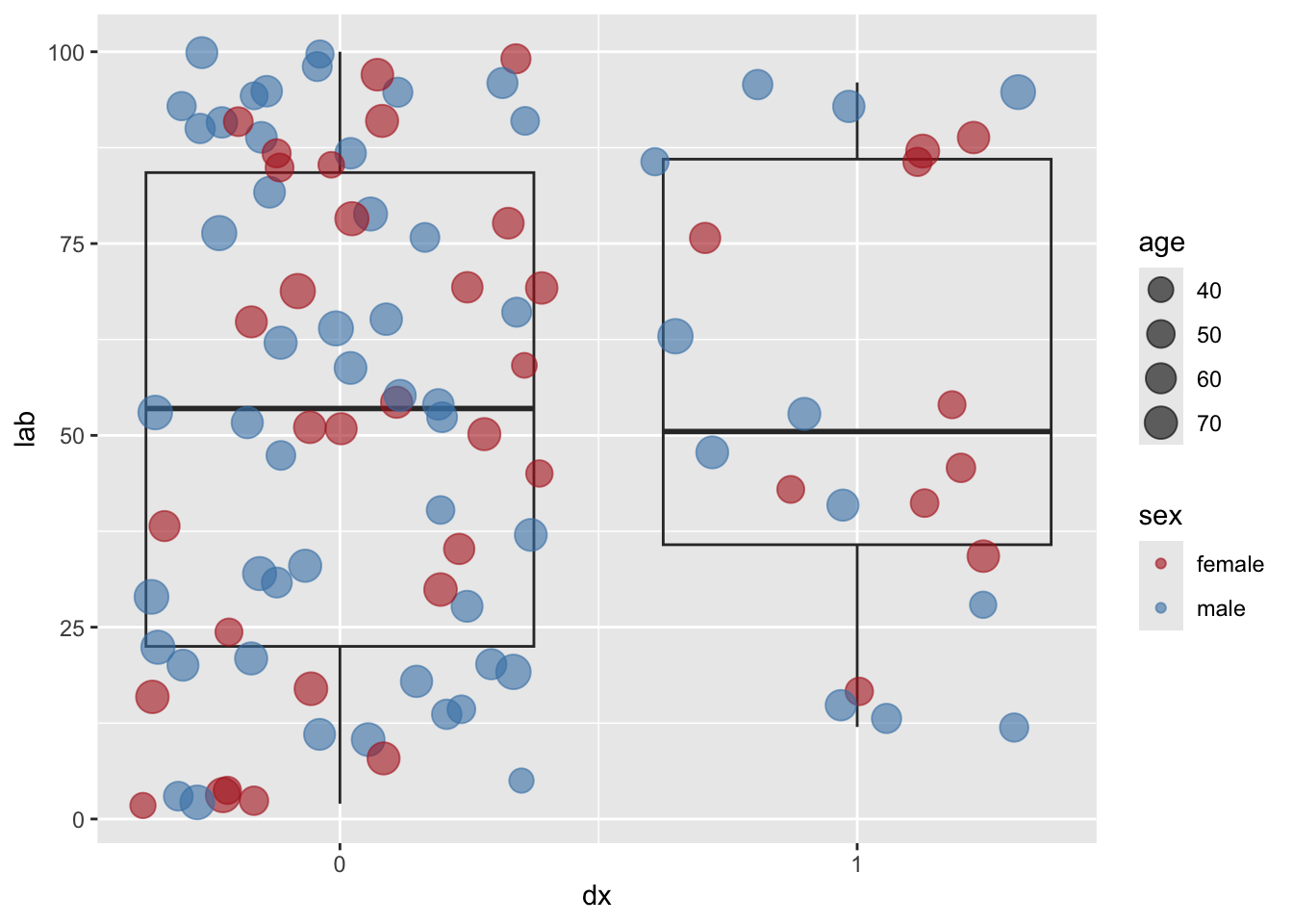

g + scale_size_continuous(range = c(4, 20))