
Color and Colorspace in ggplot2
Contents
- Introduction
- Color Models: RGB, HSV, HCL, and LUV
- R’s Color Vocabulary
- The LUV Perceptual Color Space
- The colorspace Package
- ColorBrewer in ggplot2
- Color Harmony — Building Matched Sets
- Project Palettes — Named Swatches with Hex IDs
- Using Palettes in ggplot2
- Summary
1. Introduction
Color is one of the most powerful — and most misused — channels in data visualization. Used well it guides attention, encodes magnitude, and groups categories. Used carelessly it misleads, confuses colorblind readers, and looks garish in print.
This post covers the theory first (why different color spaces exist), then the practical tools R provides, and ends with a set of named, hex-tagged project palettes you can copy into any ggplot2 project.
2. Color Models: RGB, HSV, HCL, and LUV
2.1 RGB — What Computers See
Every color on screen is an additive mixture of Red, Green, and Blue
light. Values run 0–255 (or 0–1) per channel. RGB is perfect for
rendering but terrible for human reasoning: #1A6FAD and
#5B9DC9 look nothing like “the same blue at different
brightness” even though they are.
2.2 HSV — Artist’s Intuition
Hue–Saturation–Value rearranges RGB into something more intuitive:
| Dimension | Range | Meaning |
|---|---|---|
| H Hue | 0–360° | Position on the color wheel (red → green → blue → back) |
| S Saturation | 0–1 | Grey (0) to pure color (1) |
| V Value | 0–1 | Black (0) to full brightness (1) |
HSV is better than RGB for picking colors by hand but is not perceptually uniform — equal steps in HSV do not look equal to the human eye.
2.3 HCL — Perceptually Uniform and Human-Friendly
Hue–Chroma–Luminance is the gold standard for data visualization:
| Dimension | Meaning |
|---|---|
| H Hue | Same as HSV: angle on the color wheel |
| C Chroma | Colorfulness (perceptual equivalent of saturation) |
| L Luminance | Perceived brightness (not the same as RGB brightness) |
Equal steps in HCL look equal to human eyes. This means palettes built in HCL space automatically have balanced visual weight across colors.
2.4 LUV (CIELUV) — The Math Behind HCL
HCL is the polar form of the CIELUV color space. LUV uses Cartesian coordinates (L, U, V) where L is luminance and the (U, V) plane encodes chromaticity. We will plot all of R’s 657 named colors in this space in Section 4.
3. R’s Color Vocabulary
3.1 Named Colors
# R has 657 named colors
length(colors())
## [1] 657head(colors(), 20)## [1] "white" "aliceblue" "antiquewhite" "antiquewhite1"
## [5] "antiquewhite2" "antiquewhite3" "antiquewhite4" "aquamarine"
## [9] "aquamarine1" "aquamarine2" "aquamarine3" "aquamarine4"
## [13] "azure" "azure1" "azure2" "azure3"
## [17] "azure4" "beige" "bisque" "bisque1"3.2 Hex Codes and Conversion
# Hex → RGB
col2rgb("#268bd2")
## [,1]
## red 38
## green 139
## blue 210# RGB → Hex
rgb(38, 139, 210, maxColorValue = 255)## [1] "#268BD2"# Named color → Hex
col2rgb("steelblue")## [,1]
## red 70
## green 130
## blue 180# HSV → Hex
hsv(h = 0.61, s = 0.73, v = 0.82)## [1] "#386CD1"# HCL → Hex (base R)
hcl(h = 220, c = 80, l = 55)## [1] "#0097C1"3.3 Plotting Named Colors by Hue
R’s 657 named colors sorted by Hue–Saturation–Value:
set_text_contrast <- function(color) {
  avg <- mean(col2rgb(color))
  ifelse(avg > 127, "black", "white")
}

txt_contrast <- sapply(colors(), set_text_contrast)

rgb_mat   <- col2rgb(colors())
hsv_mat   <- rgb2hsv(rgb_mat[1,], rgb_mat[2,], rgb_mat[3,], maxColorValue = 255)
hue_order <- order(hsv_mat[1,], hsv_mat[2,], hsv_mat[3,])

col_count <- 15
row_count <- ceiling(length(colors()) / col_count)

plot(0, type = "n", axes = FALSE, xlab = "", ylab = "",
     xlim = c(0.5, col_count + 0.5), ylim = c(row_count + 0.5, 0.5))
title("R Named Colors — Sorted by Hue, Saturation, Value", cex.main = 0.9)

for (j in seq(0, row_count - 1)) {
  for (i in seq(1, col_count)) {
    k <- j * col_count + i
    if (k <= length(colors())) {
      idx <- hue_order[k]
      rect(i - 0.5, j + 0.5, i + 0.5, j - 0.5,
           col = colors()[idx], border = NA)
      text(i, j, idx, cex = 0.35, col = txt_contrast[idx])
    }
  }
}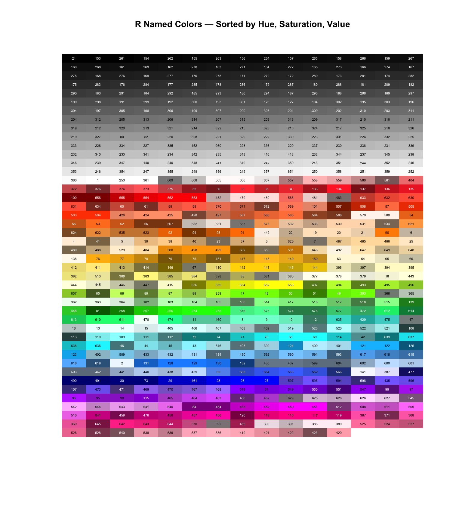
The index number shown on each tile is its position in
colors() — use colors()[n] to retrieve any
color by index.
4. The LUV Perceptual Color Space
Plotting all named R colors in CIELUV space reveals the geometry of human color perception. The horizontal U axis runs roughly green → red; the vertical V axis runs blue → yellow. Colors that look similar are close together; colors that are perceptually distant are far apart.
library(ggplot2)

# Convert all named colors to LUV via grDevices
rgb_mat <- t(col2rgb(colors())) / 255
luv_mat <- convertColor(rgb_mat, from = "sRGB", to = "Luv",
                         to.ref.white = "D65")
luv_df  <- data.frame(L = luv_mat[,1], U = luv_mat[,2], V = luv_mat[,3],
                       col = colors())

ggplot(luv_df, aes(x = U, y = V)) +
  geom_point(color = luv_df$col, size = 6, alpha = 0.75) +
  labs(
    title    = "R Named Colors in CIELUV Space",
    subtitle = "Each point colored with the color it represents",
    x        = "U  (green ← → red)",
    y        = "V  (blue ← → yellow)"
  ) +
  theme_gray(base_size = 13)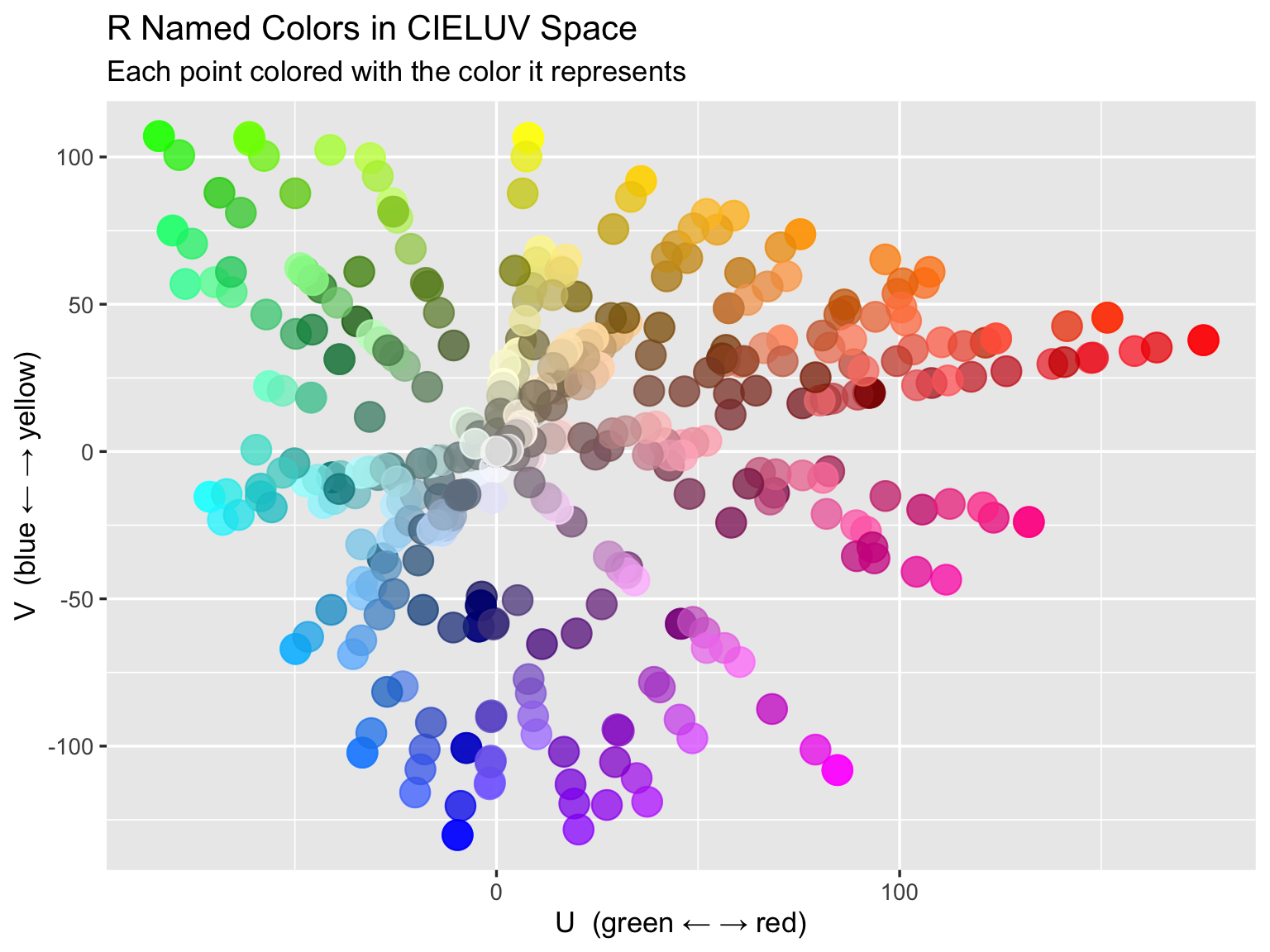
Notice how saturated colors cluster near the origin, while the colorful hues fan outward. White, grays, and black all sit at (U=0, V=0), since they have zero chrominance.
5. The colorspace Package
The colorspace package provides perceptually-grounded
palette generators directly in HCL space. It generates three palette
families that match three data types:
| Palette family | Data type | Example function |
|---|---|---|
| Qualitative | Unordered categories | qualitative_hcl(n) |
| Sequential | Ordered low → high | sequential_hcl(n) |
| Diverging | Ordered around a midpoint | diverging_hcl(n) |
library(colorspace)

par(mfrow = c(3, 1), mar = c(1, 4, 2, 1))

# Qualitative: equal C and L, evenly-spaced hues
barplot(rep(1, 8), col = qualitative_hcl(8, palette = "Dark 3"),
        border = NA, main = "Qualitative — Dark 3  (categorical data)", axes = FALSE)

# Sequential: fixed hue, varying C and L
barplot(rep(1, 9), col = sequential_hcl(9, palette = "Blues 3"),
        border = NA, main = "Sequential — Blues 3  (ordered data)", axes = FALSE)

# Diverging: two hues meeting at a neutral midpoint
barplot(rep(1, 11), col = diverging_hcl(11, palette = "Blue-Red 2"),
        border = NA, main = "Diverging — Blue-Red 2  (data centred at zero)", axes = FALSE)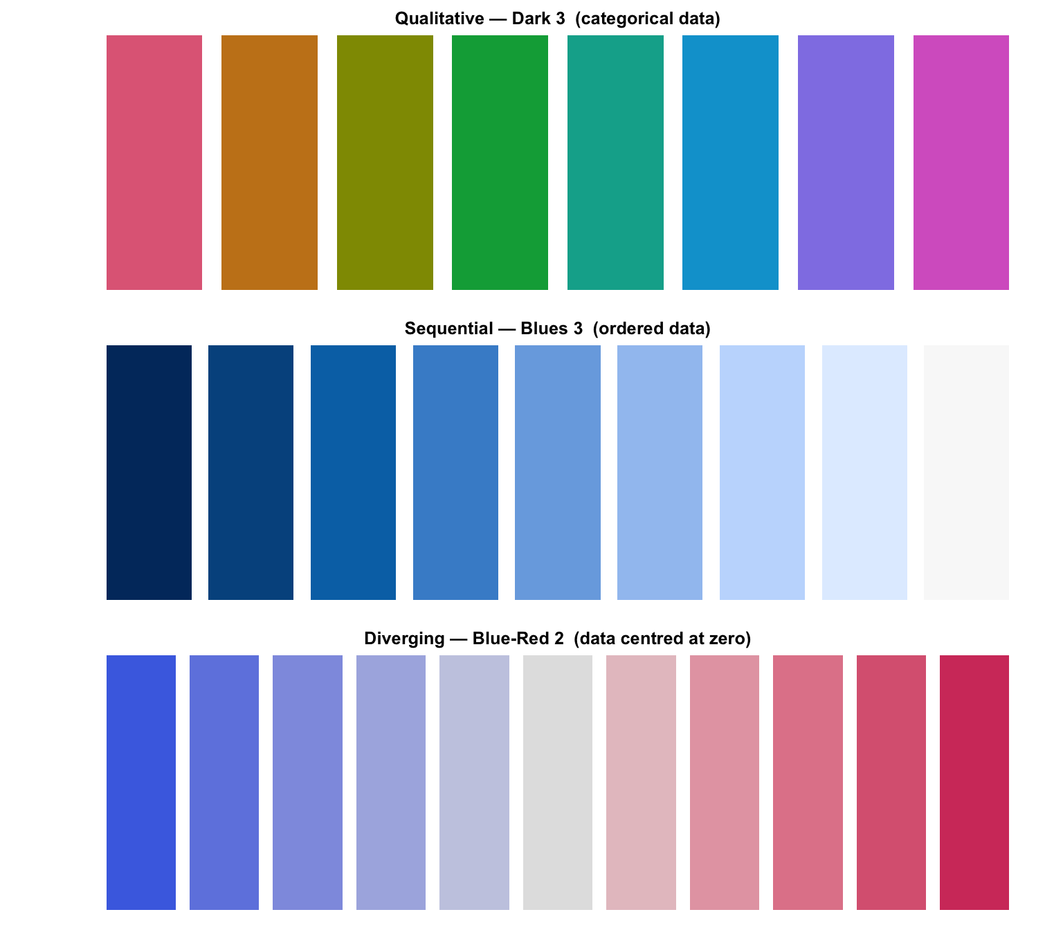
par(mfrow = c(1, 1))Using colorspace in ggplot2
library(dplyr)

# qualitative: scale_color_discrete_qualitative()
# sequential:  scale_fill_continuous_sequential()
# diverging:   scale_fill_continuous_diverging()

set.seed(1)
demo_df <- data.frame(
  x     = rnorm(120),
  y     = rnorm(120),
  group = rep(LETTERS[1:6], 20),
  value = rnorm(120)
)

ggplot(demo_df, aes(x = x, y = y, color = group)) +
  geom_point(size = 2.5, alpha = 0.8) +
  scale_color_discrete_qualitative(palette = "Dark 3") +
  labs(title = "qualitative_hcl via scale_color_discrete_qualitative()",
       color = "Group") +
  theme_gray(base_size = 13)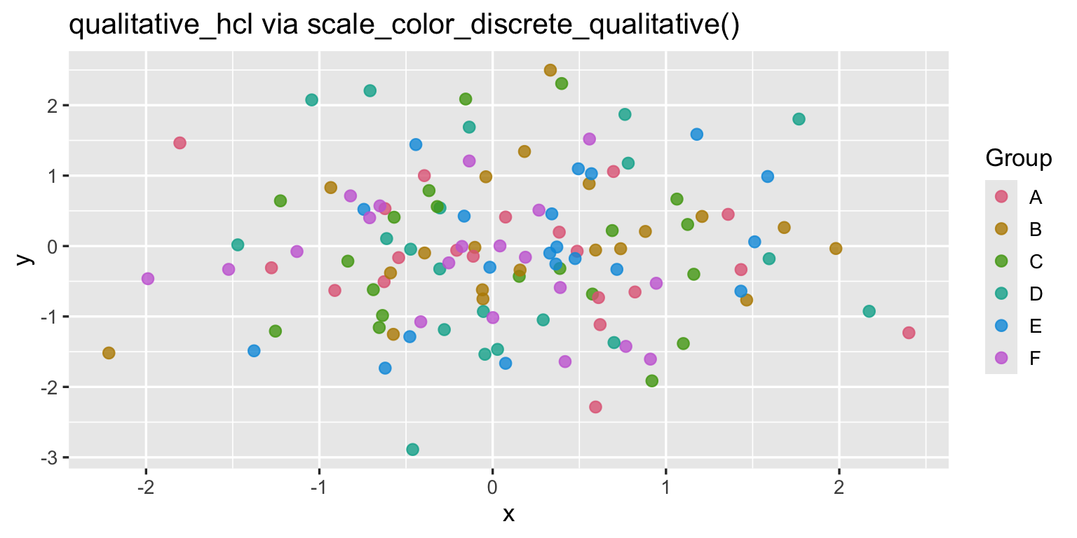
You can inspect any palette’s HCL trajectory with
specplot():
specplot(sequential_hcl(9, "Blues 3"), asp = 1/3)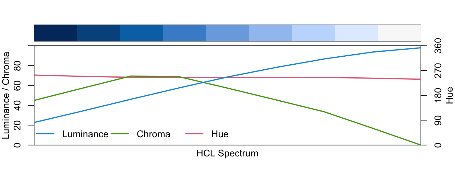
The three lines show Hue (H), Chroma (C), and Luminance (L) as the palette progresses. A good sequential palette has monotonically increasing L and decreasing C — this is what makes it readable in grayscale.
6. ColorBrewer in ggplot2
ColorBrewer (Cynthia Brewer, Penn State) provides hand-tuned palettes originally designed for cartography. They are colorblind-safe, print-safe, and photocopy-safe.
library(RColorBrewer)
display.brewer.all()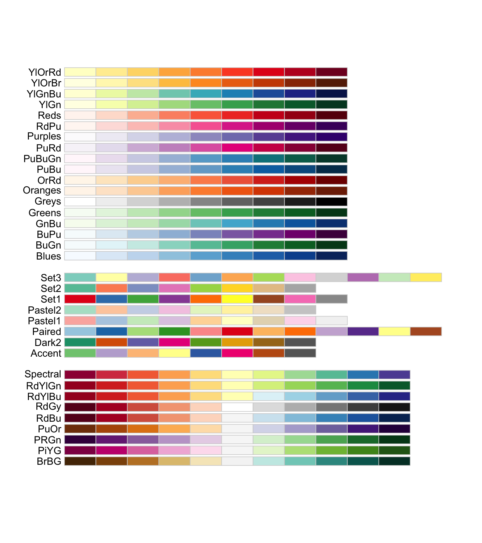
Key ggplot2 scales
# Qualitative fill: scale_fill_brewer(palette = "Set2")
# Sequential fill:  scale_fill_distiller(palette = "Blues")
# Diverging fill:   scale_fill_distiller(palette = "RdBu")

ggplot(demo_df, aes(x = x, y = y, color = group)) +
  geom_point(size = 2.5, alpha = 0.85) +
  scale_color_brewer(palette = "Set2") +
  labs(title = "ColorBrewer Set2 — scale_color_brewer(palette = 'Set2')",
       color = "Group") +
  theme_gray(base_size = 13)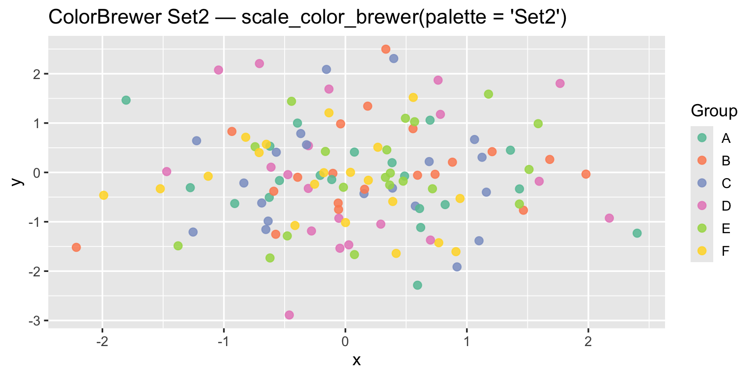
Choosing a ColorBrewer palette
# Which palettes are colorblind-safe?
subset(brewer.pal.info, colorblind == TRUE)
## maxcolors category colorblind
## BrBG 11 div TRUE
## PiYG 11 div TRUE
## PRGn 11 div TRUE
## PuOr 11 div TRUE
## RdBu 11 div TRUE
## RdYlBu 11 div TRUE
## Dark2 8 qual TRUE
## Paired 12 qual TRUE
## Set2 8 qual TRUE
## Blues 9 seq TRUE
## BuGn 9 seq TRUE
## BuPu 9 seq TRUE
## GnBu 9 seq TRUE
## Greens 9 seq TRUE
## Greys 9 seq TRUE
## Oranges 9 seq TRUE
## OrRd 9 seq TRUE
## PuBu 9 seq TRUE
## PuBuGn 9 seq TRUE
## PuRd 9 seq TRUE
## Purples 9 seq TRUE
## RdPu 9 seq TRUE
## Reds 9 seq TRUE
## YlGn 9 seq TRUE
## YlGnBu 9 seq TRUE
## YlOrBr 9 seq TRUE
## YlOrRd 9 seq TRUE7. Color Harmony — Building Matched Sets
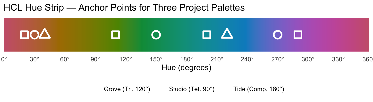
Color harmony describes combinations of hues that are visually pleasing and functionally distinct. All systems below work in HCL hue space (0–360°).
7.1 The HCL Hue Strip
library(tidyr)

h_vals <- seq(0, 360, length.out = 721)
fills  <- hcl(h_vals, c = 70, l = 55)
fills[is.na(fills)] <- "#AAAAAA"

strip_df <- data.frame(h = h_vals, fill = fills)

# Anchor points for the three palettes defined in Section 8
harm_df <- data.frame(
  h       = c(220, 40,                   # Tide: complementary
               30,  150, 270,             # Grove: triadic
               20,  110, 200, 290),       # Studio: tetradic
  palette = c(rep("Tide (Comp. 180°)", 2),
              rep("Grove (Tri. 120°)",  3),
              rep("Studio (Tet. 90°)",  4))
)

ggplot() +
  geom_tile(data = strip_df,
            aes(x = h, y = 0, fill = fill), width = 0.5, height = 0.55) +
  geom_point(data = harm_df,
             aes(x = h, y = 0, shape = palette),
             size = 4.5, color = "white", stroke = 1.8) +
  scale_fill_identity() +
  scale_x_continuous(breaks = seq(0, 360, 30),
                     labels = paste0(seq(0, 360, 30), "°"),
                     expand = c(0, 0)) +
  scale_shape_manual(values = c(21, 22, 24)) +
  labs(title = "HCL Hue Strip — Anchor Points for Three Project Palettes",
       x = "Hue (degrees)", shape = NULL) +
  theme_minimal(base_size = 12) +
  theme(
    axis.title.y    = element_blank(),
    axis.text.y     = element_blank(),
    panel.grid      = element_blank(),
    legend.position = "bottom"
  )
7.2 Complementary — 2 Hues, 180° Apart
Maximum contrast. Ideal for binary comparisons (treated vs control, before vs after). Risk of visual vibration when used at full saturation — reduce chroma or luminance on one member.
7.3 Triadic — 3 Hues, 120° Apart
Balanced and vibrant. Good for three-category data. All three hues share the same HCL chroma and luminance so no color dominates.
7.4 Tetradic (Square) — 4 Hues, 90° Apart
Rich four-color palettes. Harder to balance — typically keep chroma moderate (50–65) to avoid visual noise. One color should dominate and the others support.
7.5 Analogous — Adjacent Hues (30–60° Apart)
Low contrast, high harmony. Good for backgrounds, shading, or when you need many steps of the same “temperature.” Not suitable as a qualitative palette because the colors are too similar.
8. Project Palettes — Named Swatches with Hex IDs
Three ready-to-use palettes, each generated in HCL space with equal chroma and luminance so the colors have balanced visual weight.
# All generated with grDevices::hcl(h, c, l)
# Equal C and L within each palette = equal perceptual weight

# --- Tide: Complementary (H = 220° blue  ↔  40° amber) ---
tide <- c(
  tide_deep  = hcl(220, 80, 42),
  tide_mid   = hcl(220, 50, 62),
  tide_amber = hcl( 40, 80, 55),
  tide_gold  = hcl( 40, 45, 73)
)

# --- Grove: Triadic (H = 30°, 150°, 270°, 120° steps) ---
grove <- c(
  grove_copper = hcl( 30, 68, 52),
  grove_fern   = hcl(150, 58, 52),
  grove_violet = hcl(270, 55, 45)
)

# --- Studio: Tetradic (H = 20°, 110°, 200°, 290°, 90° steps) ---
studio <- c(
  studio_coral  = hcl( 20, 68, 52),
  studio_olive  = hcl(110, 52, 55),
  studio_steel  = hcl(200, 62, 48),
  studio_plum   = hcl(290, 52, 45)
)

# Print hex codes for reference
cat("=== Tide (Complementary) ===\n")
## === Tide (Complementary) ===print(toupper(tide))## tide_deep tide_mid tide_amber tide_gold
## "#0078A1" "#3DA2BD" "#BD7214" "#DAA989"cat("\n=== Grove (Triadic) ===\n")##
## === Grove (Triadic) ===print(toupper(grove))## grove_copper grove_fern grove_violet
## "#B56841" "#00905E" "#6B62A6"cat("\n=== Studio (Tetradic) ===\n")##
## === Studio (Tetradic) ===print(toupper(studio))## studio_coral studio_olive studio_steel studio_plum
## "#BA6453" "#6B8E3D" "#008690" "#85599E"# Helper: luminance-based text contrast
contrast_col <- function(hex) {
rgb_v <- col2rgb(hex)
lum <- (0.299 * rgb_v[1,] + 0.587 * rgb_v[2,] + 0.114 * rgb_v[3,]) / 255
ifelse(lum > 0.48, "#222222", "#FFFFFF")
}
draw_swatches <- function(palettes, title = "Project Palettes") {
df <- lapply(names(palettes), function(pname) {
cols <- palettes[[pname]]
data.frame(
palette = pname,
col_name = names(cols),
hex = toupper(cols),
fill = as.character(cols),
x = seq_along(cols),
stringsAsFactors = FALSE
)
}) |> bind_rows()
df$txt_col <- contrast_col(df$fill)
ggplot(df, aes(x = x, y = 0)) +
geom_tile(aes(fill = fill), width = 0.95, height = 0.8) +
geom_text(aes(label = col_name, color = txt_col),
vjust = -0.25, size = 3.4, fontface = "bold") +
geom_text(aes(label = hex, color = txt_col),
vjust = 1.6, size = 3.0, family = "mono") +
scale_fill_identity() +
scale_color_identity() +
scale_x_continuous(breaks = NULL) +
scale_y_continuous(breaks = NULL, expand = expansion(mult = 0.6)) +
facet_wrap(~ palette, ncol = 1, scales = "free_x") +
labs(title = title) +
theme_void(base_size = 12) +
theme(
strip.text = element_text(face = "bold", size = 12, hjust = 0,
margin = margin(b = 4, t = 10)),
panel.spacing = unit(1.5, "lines"),
plot.title = element_text(face = "bold", size = 14,
margin = margin(b = 10))
)
}all_palettes <- list(
"Tide — Complementary (H: 220° / 40°)" = tide,
"Grove — Triadic (H: 30° / 150° / 270°)" = grove,
"Studio — Tetradic (H: 20° / 110° / 200° / 290°)" = studio
)
draw_swatches(all_palettes)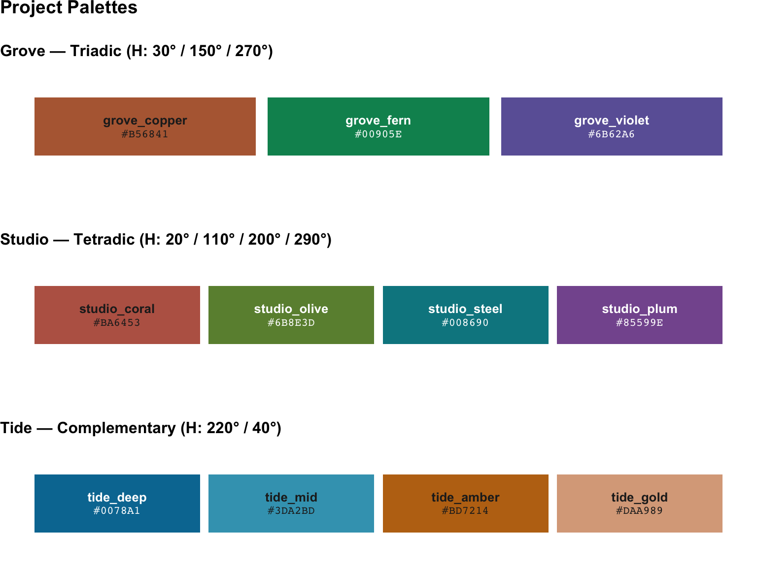
Quick-reference table
| Palette | Name | Hex | Harmony | H. | C | L | |
|---|---|---|---|---|---|---|---|
| tide_deep | Tide | tide_deep | #0078A1 | Complementary | 220 | 80 | 42 |
| tide_mid | Tide | tide_mid | #3DA2BD | Complementary | 220 | 50 | 62 |
| tide_amber | Tide | tide_amber | #BD7214 | Complementary | 40 | 80 | 55 |
| tide_gold | Tide | tide_gold | #DAA989 | Complementary | 40 | 45 | 73 |
| grove_copper | Grove | grove_copper | #B56841 | Triadic | 30 | 68 | 52 |
| grove_fern | Grove | grove_fern | #00905E | Triadic | 150 | 58 | 52 |
| grove_violet | Grove | grove_violet | #6B62A6 | Triadic | 270 | 55 | 45 |
| studio_coral | Studio | studio_coral | #BA6453 | Tetradic | 20 | 68 | 52 |
| studio_olive | Studio | studio_olive | #6B8E3D | Tetradic | 110 | 52 | 55 |
| studio_steel | Studio | studio_steel | #008690 | Tetradic | 200 | 62 | 48 |
| studio_plum | Studio | studio_plum | #85599E | Tetradic | 290 | 52 | 45 |
9. Using Palettes in ggplot2
9.1 Qualitative — scale_color_manual() /
scale_fill_manual()
# Three-group example using Grove (triadic)
set.seed(7)
df3 <- data.frame(
  x     = rnorm(90),
  y     = rnorm(90),
  group = rep(c("Alpha", "Beta", "Gamma"), 30)
)

ggplot(df3, aes(x = x, y = y, color = group)) +
  geom_point(size = 3, alpha = 0.85) +
  scale_color_manual(values = unname(grove)) +
  labs(title = "Grove palette — scale_color_manual(values = unname(grove))",
       color = "Group") +
  theme_gray(base_size = 13)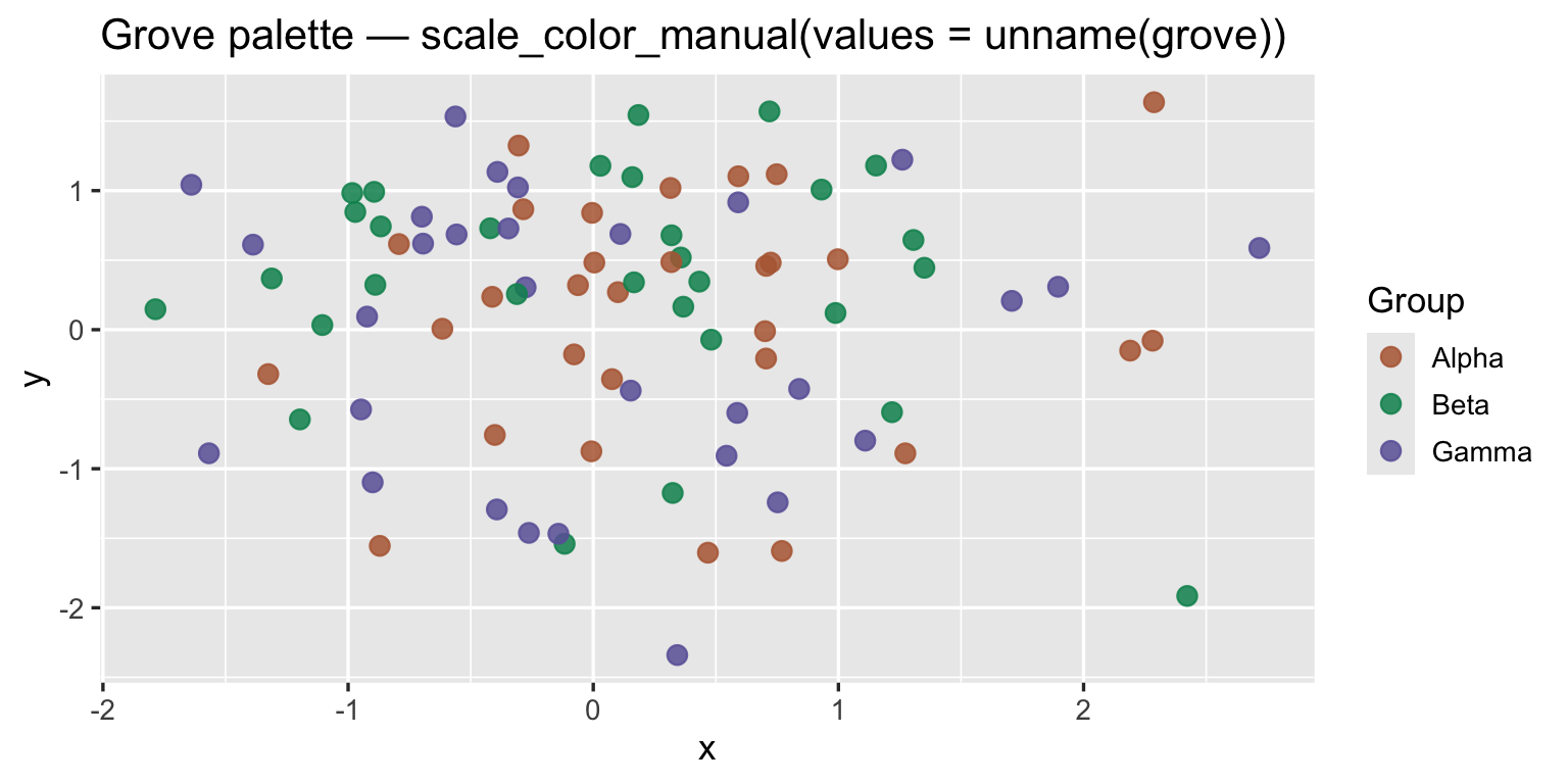
9.2 Two-Group Contrast — Tide Complementary Pair
df2 <- data.frame(
  group = rep(c("Control", "Treated"), each = 40),
  value = c(rnorm(40, 10, 2), rnorm(40, 13, 2.5))
)

ggplot(df2, aes(x = group, y = value, fill = group)) +
  geom_boxplot(alpha = 0.85, width = 0.5) +
  geom_jitter(aes(color = group), width = 0.12, size = 1.8, alpha = 0.6) +
  scale_fill_manual(values  = c(Control = tide[["tide_mid"]],
                                Treated = tide[["tide_amber"]])) +
  scale_color_manual(values = c(Control = tide[["tide_deep"]],
                                Treated = tide[["tide_gold"]])) +
  labs(title = "Tide palette — complementary pair for binary comparison") +
  guides(fill = "none", color = "none") +
  theme_gray(base_size = 13)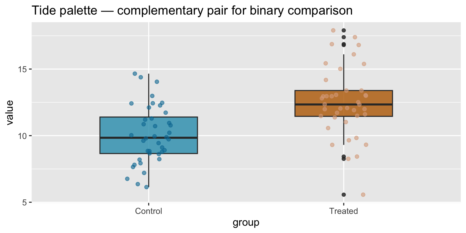
9.3 Four-Category — Studio Tetradic
df4 <- data.frame(
  category = rep(c("Q1", "Q2", "Q3", "Q4"), each = 30),
  x        = rnorm(120),
  y        = c(rnorm(30, 1), rnorm(30, -1), rnorm(30, 1, 0.5), rnorm(30, -0.5))
)

ggplot(df4, aes(x = x, y = y, color = category)) +
  geom_point(size = 2.5, alpha = 0.8) +
  scale_color_manual(values = unname(studio)) +
  labs(title = "Studio palette — scale_color_manual(values = unname(studio))",
       color = "Quarter") +
  theme_gray(base_size = 13)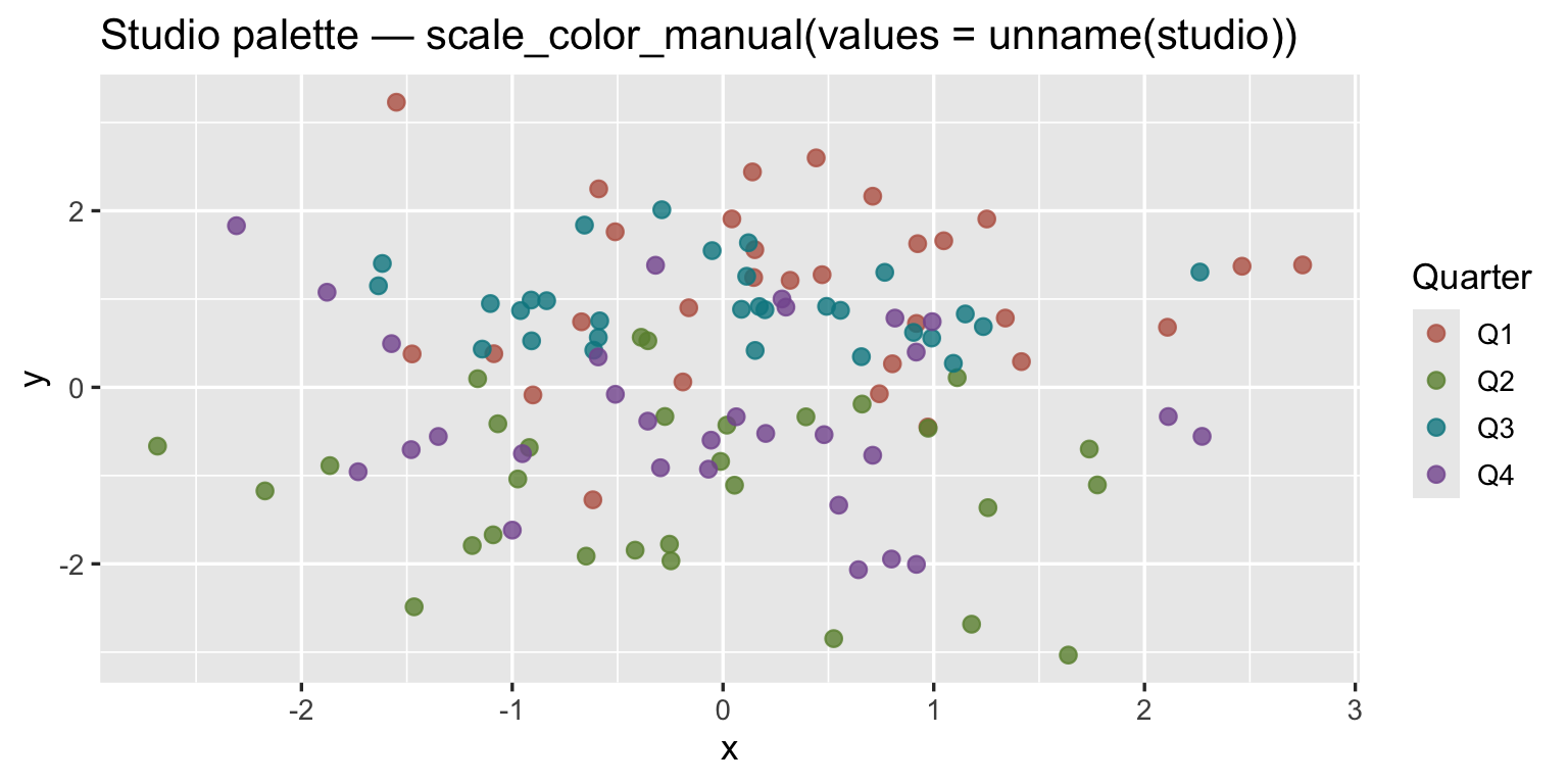
9.4 Storing Palettes for Reuse
Define your palettes once in a project-level colors.R
file and source() it at the top of each script:
# colors.R — project palette definitions

tide <- c(
  tide_deep  = "#1B4E8A",   # adjust to your actual hex values
  tide_mid   = "#4A82B8",
  tide_amber = "#C96A1A",
  tide_gold  = "#E8AB68"
)

grove <- c(
  grove_copper = "#A84C25",
  grove_fern   = "#2D7A52",
  grove_violet = "#4D3B8C"
)

studio <- c(
  studio_coral = "#B54230",
  studio_olive = "#5E7A2A",
  studio_steel = "#1E5E88",
  studio_plum  = "#5A3576"
)
10. Summary
| Topic | Key points |
|---|---|
| Color models | RGB for rendering; HSV for intuition; HCL for perceptual balance; LUV is HCL’s Cartesian parent |
| HCL | Equal C and L = equal visual weight; hue angle drives harmony |
colorspace |
qualitative_hcl, sequential_hcl,
diverging_hcl for the three data types; drop-in ggplot2
scales |
| ColorBrewer | Hand-tuned, colorblind/print-safe; scale_color_brewer()
/ scale_fill_distiller() |
| Harmony types | Complementary (180°, binary contrast), Triadic (120°, 3-way balance), Tetradic (90°, 4-way); Analogous (adjacent, low contrast) |
| Project palettes | Tide (blue/amber, 2+2), Grove (copper/fern/violet, 3), Studio (coral/olive/steel/plum, 4) |
| In ggplot2 | scale_color_manual(values = palette_vector) — name the
vector elements to match factor levels |