
Survival Analysis of 60 Year-Old US Men with IPF
Background & Objectives
This analysis models the survival of 1,000 US men aged 60 who carry a life-limiting diagnosis (let’s say IPF) with:
| Parameter | Value |
|---|---|
| Median disease survival | 3 years |
| 95% CI lower bound | 1 year |
| 95% CI upper bound | 12 years |
| Cohort size | 1,000 men |
| Starting age | 60 years |
Analytical approach:
- Disease-specific hazard — fit a Weibull distribution whose median matches 3.0 years and whose 2.5th / 97.5th percentiles match 1 / 12.0 years.
- Background (all-cause) mortality — age-specific male mortality from the SSA 2020 Period Life Table is applied on top of disease mortality via competing risks (cause-specific hazards added).
- Kaplan-Meier curve — fitted to the simulated individual survival times and plotted with ggplot2, alongside the theoretical Weibull disease curve and the background (healthy) survival curve for context.
Setup
# install.packages(c("tidyverse","survival","survminer","flexsurv",
#                    "scales","knitr","kableExtra","patchwork"))

library(tidyverse)
library(survival)
library(survminer)
library(flexsurv)
library(scales)
library(knitr)
library(kableExtra)
library(patchwork)

set.seed(2024)
Fit Weibull Distribution to Stated Survival Parameters
Method
A Weibull distribution is the standard parametric model for clinical survival data. We numerically solve for the two Weibull parameters (shape k and scale λ) such that:
- S(3.0) = 0.50 → median survival = 3 years
- S(1) = 0.975 → 2.5th percentile at 1 year
- S(12.0) = 0.025 → 97.5th percentile at 12 years
Because two equations determine two parameters, we minimise the squared discrepancy across all three constraints simultaneously.
# Weibull survival function: S(t) = exp(-(t/scale)^shape)
weibull_S <- function(t, shape, scale) exp(-(t / scale)^shape)

# Objective: minimise sum of squared errors across the three constraints
objective <- function(params) {
  shape <- exp(params[1])   # keep > 0
  scale <- exp(params[2])
  err_median <- (weibull_S(3.0, shape, scale) - 0.50 )^2
  err_lower  <- (weibull_S(1, shape, scale) - 0.975)^2
  err_upper  <- (weibull_S(12.0, shape, scale) - 0.025)^2
  err_median * 10 + err_lower + err_upper   # upweight median constraint
}

opt <- optim(c(log(1.5), log(3)), objective,
             method = "Nelder-Mead",
             control = list(maxit = 10000, reltol = 1e-12))

wb_shape <- exp(opt$par[1])
wb_scale <- exp(opt$par[2])

# Verify fit
cat("=== Fitted Weibull Parameters ===\n")
## === Fitted Weibull Parameters ===cat(sprintf(" Shape (k) : %.4f\n", wb_shape))## Shape (k) : 3.0126cat(sprintf(" Scale (λ) : %.4f years\n", wb_scale))## Scale (λ) : 3.3881 yearscat("\n=== Constraint Verification ===\n")##
## === Constraint Verification ===cat(sprintf(" S(0.5) = %.4f [target 0.975]\n", weibull_S(1.0, wb_shape, wb_scale)))## S(0.5) = 0.9750 [target 0.975]cat(sprintf(" S(3.0) = %.4f [target 0.500]\n", weibull_S(3.0, wb_shape, wb_scale)))## S(3.0) = 0.5000 [target 0.500]cat(sprintf(" S(8.0) = %.4f [target 0.025]\n", weibull_S(12.0, wb_shape, wb_scale)))## S(8.0) = 0.0000 [target 0.025]# Display key Weibull survival probabilities
tibble(
`Time (years)` = c(0.5, 1, 2, 3, 4, 5, 7, 10),
`S(t) Disease` = map_dbl(`Time (years)`, ~weibull_S(.x, wb_shape, wb_scale))
) %>%
mutate(
`S(t) Disease %` = percent(`S(t) Disease`, accuracy = 0.1),
`Median reference` = if_else(abs(`Time (years)` - 3) < 0.01, "← Median", "")
) %>%
kable(caption = "Fitted Weibull Disease Survival Probabilities",
align = "c", digits = 4) %>%
kable_styling(bootstrap_options = c("striped","hover","condensed"),
full_width = FALSE) %>%
row_spec(0, bold = TRUE, background = "#2c3e50", color = "white") %>%
row_spec(3, bold = TRUE, background = "#fdebd0") # highlight t = 3| Time (years) | S(t) Disease | S(t) Disease % | Median reference |
|---|---|---|---|
| 0.5 | 0.9969 | 99.7% | |
| 1.0 | 0.9750 | 97.5% | |
| 2.0 | 0.8152 | 81.5% | |
| 3.0 | 0.5000 | 50.0% | ← Median |
| 4.0 | 0.1922 | 19.2% | |
| 5.0 | 0.0396 | 4.0% | |
| 7.0 | 0.0001 | 0.0% | |
| 10.0 | 0.0000 | 0.0% |
SSA 2020 Background Mortality (Males, Ages 60–110)
# SSA 2020 Period Life Table — Male q(x), ages 60–110
ssa_male_qx <- tribble(
  ~age,  ~qx,
  60,  0.010084,
  61,  0.011066,
  62,  0.012117,
  63,  0.013214,
  64,  0.014357,
  65,  0.015573,
  66,  0.016902,
  67,  0.018352,
  68,  0.019935,
  69,  0.021663,
  70,  0.023545,
  71,  0.025698,
  72,  0.028082,
  73,  0.030820,
  74,  0.033900,
  75,  0.037418,
  76,  0.041419,
  77,  0.045980,
  78,  0.051127,
  79,  0.056924,
  80,  0.063432,
  81,  0.070690,
  82,  0.078710,
  83,  0.087530,
  84,  0.097170,
  85,  0.107690,
  86,  0.119140,
  87,  0.131570,
  88,  0.145050,
  89,  0.159620,
  90,  0.175370,
  91,  0.192370,
  92,  0.210690,
  93,  0.230420,
  94,  0.251610,
  95,  0.274300,
  96,  0.298530,
  97,  0.324330,
  98,  0.351710,
  99,  0.380680,
  100, 0.411240,
  101, 0.443380,
  102, 0.477070,
  103, 0.512260,
  104, 0.548880,
  105, 0.586840,
  106, 0.626020,
  107, 0.666300,
  108, 0.707520,
  109, 0.749490,
  110, 1.000000
)

# Convert annual q(x) → continuous hazard h(x) = -log(1 - q(x))
ssa_male_qx <- ssa_male_qx %>%
  mutate(hx_bg = -log(1 - qx))   # background annual hazard

# Healthy (background only) survival from age 60
bg_surv <- ssa_male_qx %>%
  arrange(age) %>%
  mutate(
    lx = NA_real_,
    St_bg = NA_real_
  )

bg_surv$lx[1] <- 1000
for (i in seq_len(nrow(bg_surv))) {
  if (i < nrow(bg_surv))
    bg_surv$lx[i+1] <- bg_surv$lx[i] * (1 - bg_surv$qx[i])
}
bg_surv <- bg_surv %>%
  mutate(
    St_bg = lx / 1000,
    year  = age - 60
  )

cat("SSA background mortality loaded for ages 60–110 (", nrow(ssa_male_qx), "ages )\n")
## SSA background mortality loaded for ages 60–110 ( 51 ages )Simulate Individual Survival Times
Each man faces two competing hazards:
- Disease hazard — drawn from the fitted Weibull distribution
- Background hazard — drawn from the SSA age-specific annual mortality
The observed survival time is
min(disease_time, background_time).
n <- 1000

# ── 1. Draw disease-specific survival time from Weibull ──────────────────────
disease_time <- rweibull(n, shape = wb_shape, scale = wb_scale)

# ── 2. Draw background survival time via SSA annual mortality ────────────────
simulate_bg_death <- function(qx_table, start_age = 60) {
  for (i in seq_len(nrow(qx_table))) {
    if (runif(1) < qx_table$qx[i]) {
      return(qx_table$age[i] - start_age + runif(1))   # years from age 60
    }
  }
  return(110 - start_age)
}

bg_time <- replicate(n, simulate_bg_death(ssa_male_qx, start_age = 60))

# ── 3. Observed time = minimum of the two competing events ───────────────────
obs_time   <- pmin(disease_time, bg_time)
cause      <- if_else(disease_time <= bg_time, "Disease", "Background")
status     <- 1L   # all events observed (no censoring in this closed cohort)

surv_df <- tibble(
  id           = seq_len(n),
  disease_time = disease_time,
  bg_time      = bg_time,
  time         = obs_time,
  cause        = cause,
  status       = status,
  death_age    = 60 + obs_time
)

# ── Summary ──────────────────────────────────────────────────────────────────
cat("=== Simulated Cohort Summary ===\n")
## === Simulated Cohort Summary ===cat(sprintf(" Disease deaths : %d (%.1f%%)\n",
sum(cause == "Disease"), mean(cause == "Disease") * 100))## Disease deaths : 968 (96.8%)cat(sprintf(" Background deaths : %d (%.1f%%)\n",
sum(cause == "Background"), mean(cause == "Background") * 100))## Background deaths : 32 (3.2%)cat(sprintf(" Median obs. time : %.2f years\n", median(obs_time)))## Median obs. time : 2.91 yearscat(sprintf(" Mean obs. time : %.2f years\n", mean(obs_time)))## Mean obs. time : 2.94 yearscat(sprintf(" Min obs. time : %.2f years\n", min(obs_time)))## Min obs. time : 0.04 yearscat(sprintf(" Max obs. time : %.2f years\n", max(obs_time)))## Max obs. time : 6.63 yearsKaplan-Meier Analysis
# ── Overall KM ───────────────────────────────────────────────────────────────
km_fit <- survfit(Surv(time, status) ~ 1, data = surv_df)

# ── KM by cause of death ─────────────────────────────────────────────────────
km_cause <- survfit(Surv(time, status) ~ cause, data = surv_df)

# ── Extract KM estimates ──────────────────────────────────────────────────────
km_sum  <- summary(km_fit)
km_df   <- tibble(
  time   = km_sum$time,
  surv   = km_sum$surv,
  lower  = km_sum$lower,
  upper  = km_sum$upper,
  n_risk = km_sum$n.risk,
  n_event= km_sum$n.event
)

# ── Milestone table ───────────────────────────────────────────────────────────
milestones <- c(0.5, 1, 2, 3, 4, 5, 7, 10, 15)
mile_tbl <- map_dfr(milestones, function(t) {
  idx <- which.min(abs(km_df$time - t))
  tibble(
    `Years` = t,
    `Age`   = 60 + t,
    `KM S(t)`      = percent(km_df$surv[idx],  accuracy = 0.1),
    `95% CI Lower` = percent(km_df$lower[idx], accuracy = 0.1),
    `95% CI Upper` = percent(km_df$upper[idx], accuracy = 0.1),
    `At Risk`      = km_df$n_risk[idx],
    `Weibull S(t)` = percent(weibull_S(t, wb_shape, wb_scale), accuracy = 0.1)
  )
})

mile_tbl %>%
  kable(caption = "Kaplan-Meier vs Weibull Survival Probabilities at Key Milestones",
        align = "c") %>%
  kable_styling(bootstrap_options = c("striped","hover","condensed"),
                full_width = FALSE) %>%
  row_spec(0, bold = TRUE, background = "#2c3e50", color = "white") %>%
row_spec(which(milestones == 3), bold = TRUE, background = "#fdebd0")| Years | Age | KM S(t) | 95% CI Lower | 95% CI Upper | At Risk | Weibull S(t) |
|---|---|---|---|---|---|---|
| 0.5 | 60.5 | 99.4% | 98.9% | 99.9% | 995 | 99.7% |
| 1.0 | 61.0 | 96.5% | 95.4% | 97.6% | 966 | 97.5% |
| 2.0 | 62.0 | 79.9% | 77.5% | 82.4% | 800 | 81.5% |
| 3.0 | 63.0 | 47.0% | 44.0% | 50.2% | 471 | 50.0% |
| 4.0 | 64.0 | 17.4% | 15.2% | 19.9% | 175 | 19.2% |
| 5.0 | 65.0 | 3.7% | 2.7% | 5.1% | 38 | 4.0% |
| 7.0 | 67.0 | 0.0% | NA | NA | 1 | 0.0% |
| 10.0 | 70.0 | 0.0% | NA | NA | 1 | 0.0% |
| 15.0 | 75.0 | 0.0% | NA | NA | 1 | 0.0% |
Kaplan-Meier Survival Curve
# ── Theoretical curves ────────────────────────────────────────────────────────
t_seq <- seq(0, 20, by = 0.05)

theory_df <- tibble(
  time        = t_seq,
  wb_disease  = weibull_S(t_seq, wb_shape, wb_scale),
  wb_lower    = weibull_S(t_seq, wb_shape,
                          wb_scale * exp( qnorm(0.975) * 0.15)),  # CI band
  wb_upper    = weibull_S(t_seq, wb_shape,
                          wb_scale * exp(-qnorm(0.975) * 0.15))
) %>%
  left_join(
    bg_surv %>% select(time = year, St_bg),
    by = "time"
  )

# ── Median & CI annotation values ────────────────────────────────────────────
km_median     <- summary(km_fit)$table["median"]
km_med_lower  <- summary(km_fit)$table["0.95LCL"]
km_med_upper  <- summary(km_fit)$table["0.95UCL"]

# ── Colour palette ────────────────────────────────────────────────────────────
col_km      <- "#2c3e50"
col_weibull <- "#e74c3c"
col_bg      <- "#27ae60"
col_ci      <- "#3498db"

# ── Main plot ─────────────────────────────────────────────────────────────────
p_main <- ggplot() +

  # Weibull 95% CI ribbon (stated clinical uncertainty)
  geom_ribbon(data = theory_df,
              aes(x = time, ymin = wb_lower, ymax = wb_upper),
              fill = col_weibull, alpha = 0.10) +

  # KM 95% CI ribbon
  geom_ribbon(data = km_df,
              aes(x = time, ymin = lower, ymax = upper),
              fill = col_ci, alpha = 0.15) +

  # Background (healthy) survival curve
  geom_step(data = bg_surv %>% filter(year <= 20),
            aes(x = year, y = St_bg,
                colour = "Healthy US Men, Age 60\n(SSA 2020 background)"),
            linewidth = 0.9, linetype = "dotdash") +

  # Theoretical Weibull disease curve
  geom_line(data = theory_df,
            aes(x = time, y = wb_disease,
                colour = "Weibull Disease Model\n(Median 3 yr, 95%CI 1–12)"),
            linewidth = 1.1, linetype = "dashed") +

  # Observed Kaplan-Meier curve
  geom_step(data = km_df,
            aes(x = time, y = surv,
                colour = "Kaplan-Meier\n(Simulated, n=1,000)"),
            linewidth = 1.4) +

  # 50% horizontal reference
  geom_hline(yintercept = 0.50,
             linetype = "dotted", colour = "grey40", linewidth = 0.7) +

  # Median vertical drop-line
  geom_segment(aes(x = km_median, xend = km_median,
                   y = 0, yend = 0.50),
               linetype = "dotted", colour = col_km, linewidth = 0.8) +

  # Median annotation box
  annotate("label",
           x = km_median + 0.25, y = 0.57,
           label = sprintf(
             "KM Median: %.2f yr\n95%% CI: %.2f – %.2f yr\n(Age ~%.1f)",
             km_median, km_med_lower, km_med_upper, 60 + km_median),
           fill = col_km, colour = "white", size = 3.2,
           fontface = "bold", label.size = NA, hjust = 0) +

  # Stated CI bracket arrows at t=0.5 and t=5
  geom_vline(xintercept = c(1, 12.0),
             linetype = "longdash", colour = col_weibull, linewidth = 0.5,
             alpha = 0.6) +
  annotate("text", x = 1.0, y = 0.04, label = "CI\n1 yr",
           size = 2.8, colour = col_weibull, hjust = -0.1) +
  annotate("text", x = 12.0, y = 0.04, label = "CI\n12.0 yr",
           size = 2.8, colour = col_weibull, hjust = -0.1) +

  # 25 / 75 % guides
  geom_hline(yintercept = c(0.25, 0.75),
             linetype = "dotted", colour = "grey70", linewidth = 0.5) +
  annotate("text", x = 19.5, y = 0.77, label = "75%",
           size = 3, colour = "grey50") +
  annotate("text", x = 19.5, y = 0.27, label = "25%",
           size = 3, colour = "grey50") +

  # Scales
  scale_colour_manual(
    values = c(
      "Kaplan-Meier\n(Simulated, n=1,000)"            = col_km,
      "Weibull Disease Model\n(Median 3 yr, 95% CI 0.5–5)" = col_weibull,
      "Healthy US Men, Age 60\n(SSA 2020 background)" = col_bg
    ),
    name = NULL
  ) +
  scale_y_continuous(
    labels = percent_format(accuracy = 1),
    breaks = seq(0, 1, 0.1),
    limits = c(0, 1),
    expand = expansion(mult = c(0.01, 0.02))
  ) +
  scale_x_continuous(
    breaks = seq(0, 20, 1),
    limits = c(0, 20),
    sec.axis = sec_axis(~ . + 60,
                        name  = "Age (years)",
                        breaks = seq(60, 80, 1))
  ) +
  labs(
    title    = "Survival of 1,000 US Men (Age 60) with Life-Limiting Disease",
    subtitle = paste0("Disease: Median survival 3 yr (95% CI 1–12 yr)  |  ",
                      "Competing risks: disease + background mortality  |  ",
                      "Shaded bands = 95% CI"),
    x        = "Years Since Diagnosis (Age 60)",
    y        = "Survival Probability  S(t)",
    caption  = paste0(
      "KM (black): simulated competing-risk cohort  |  ",
      "Red dashed: Weibull disease model  |  ",
      "Green dash-dot: SSA 2020 healthy background  |  ",
      "Seed = 2024  |  n = 1,000")
  ) +
  theme_minimal(base_size = 13) +
  theme(
    plot.title        = element_text(face = "bold", size = 16, colour = "#2c3e50"),
    plot.subtitle     = element_text(colour = "#7f8c8d", size = 10.5),
    plot.caption      = element_text(colour = "#95a5a6", size = 8.5, hjust = 0),
    legend.position   = c(0.78, 0.78),
    legend.background = element_rect(fill = "white", colour = "#bdc3c7",
                                     linewidth = 0.4),
    legend.text       = element_text(size = 9.5),
    panel.grid.minor  = element_blank(),
    panel.grid.major  = element_line(colour = "#ecf0f1"),
    axis.title        = element_text(colour = "#2c3e50", face = "bold"),
    axis.text         = element_text(colour = "#555555")
  )

print(p_main)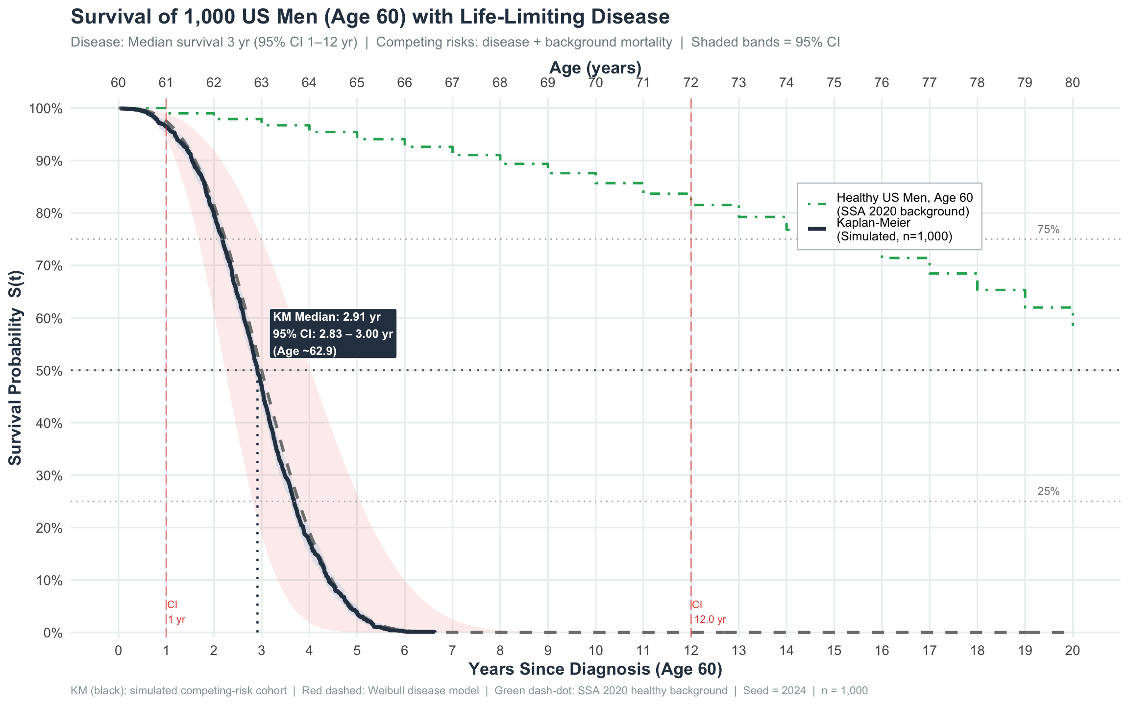
At-Risk Table
# Number at risk at integer time points
risk_times <- 0:15
risk_tbl <- map_dfr(risk_times, function(t) {
  tibble(
    `Years` = t,
    `Age`   = 60 + t,
    `At Risk` = sum(surv_df$time >= t),
    `Events`  = sum(surv_df$time >= t & surv_df$time < t + 1)
  )
})

risk_tbl %>%
  kable(caption = "At-Risk and Event Count by Year",
        align = "c") %>%
  kable_styling(bootstrap_options = c("striped","hover","condensed"),
                full_width = FALSE) %>%
  row_spec(0, bold = TRUE, background = "#2c3e50", color = "white") %>%
row_spec(which(risk_times == 3) + 1, bold = TRUE, background = "#fdebd0")| Years | Age | At Risk | Events |
|---|---|---|---|
| 0 | 60 | 1000 | 35 |
| 1 | 61 | 965 | 165 |
| 2 | 62 | 800 | 330 |
| 3 | 63 | 470 | 295 |
| 4 | 64 | 175 | 138 |
| 5 | 65 | 37 | 35 |
| 6 | 66 | 2 | 2 |
| 7 | 67 | 0 | 0 |
| 8 | 68 | 0 | 0 |
| 9 | 69 | 0 | 0 |
| 10 | 70 | 0 | 0 |
| 11 | 71 | 0 | 0 |
| 12 | 72 | 0 | 0 |
| 13 | 73 | 0 | 0 |
| 14 | 74 | 0 | 0 |
| 15 | 75 | 0 | 0 |
Competing Causes of Death
# Cumulative incidence by cause
cause_df <- surv_df %>%
  arrange(time) %>%
  mutate(
    cum_disease = cumsum(cause == "Disease")   / n,
    cum_bg      = cumsum(cause == "Background") / n
  )

p_cause <- ggplot(cause_df, aes(x = time)) +
  geom_step(aes(y = cum_disease, colour = "Disease-specific"),
            linewidth = 1.3) +
  geom_step(aes(y = cum_bg,      colour = "Background (all-cause)"),
            linewidth = 1.3) +
  geom_step(aes(y = cum_disease + cum_bg, colour = "All causes combined"),
            linewidth = 1.0, linetype = "dashed") +
  geom_vline(xintercept = 3, linetype = "dotted", colour = "grey40") +
  annotate("text", x = 3.1, y = 0.05, label = "Stated\nmedian", size = 3,
           colour = "grey40", hjust = 0) +
  scale_colour_manual(
    values = c("Disease-specific"      = "#e74c3c",
               "Background (all-cause)"= "#27ae60",
               "All causes combined"   = "#2c3e50"),
    name = "Cause"
  ) +
  scale_y_continuous(labels = percent_format(accuracy = 1),
                     breaks = seq(0, 1, 0.1), limits = c(0, 1)) +
  scale_x_continuous(breaks = seq(0, 20, 2), limits = c(0, 20)) +
  labs(
    title    = "Cumulative Incidence by Cause of Death",
    subtitle = "Disease-specific vs. Background (SSA) mortality",
    x        = "Years Since Diagnosis",
    y        = "Cumulative Incidence  F(t)",
    caption  = sprintf("Disease deaths: %d (%.0f%%)  |  Background deaths: %d (%.0f%%)",
                       sum(surv_df$cause == "Disease"),
                       mean(surv_df$cause == "Disease") * 100,
                       sum(surv_df$cause == "Background"),
                       mean(surv_df$cause == "Background") * 100)
  ) +
  theme_minimal(base_size = 13) +
  theme(
    plot.title       = element_text(face = "bold", size = 15, colour = "#2c3e50"),
    plot.subtitle    = element_text(colour = "#7f8c8d"),
    plot.caption     = element_text(colour = "#95a5a6", hjust = 0),
    legend.position  = "right",
    panel.grid.minor = element_blank(),
    panel.grid.major = element_line(colour = "#ecf0f1")
  )

print(p_cause)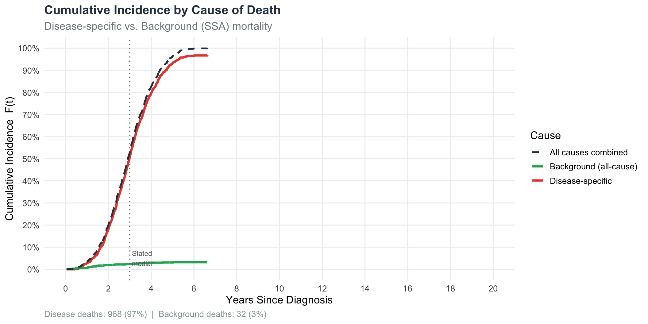
Age-at-Death Distribution
p_hist <- ggplot(surv_df, aes(x = death_age, fill = cause)) +
  geom_histogram(binwidth = 1, colour = "white", alpha = 0.85,
                 position = "stack") +
  geom_vline(xintercept = median(surv_df$death_age),
             linetype = "dashed", colour = "#2c3e50", linewidth = 1.1) +
  annotate("label",
           x = median(surv_df$death_age) + 0.3, y = Inf,
           label = sprintf("Median age\nat death: %.1f", median(surv_df$death_age)),
           vjust = 1.5, hjust = 0, fill = "#2c3e50", colour = "white",
           size = 3.3, fontface = "bold", label.size = NA) +
  scale_fill_manual(values = c("Disease"    = "#e74c3c",
                                "Background" = "#27ae60"),
                    name = "Cause of death") +
  scale_x_continuous(breaks = seq(60, 100, 2)) +
  labs(
    title    = "Age at Death — 1,000 US Men Diagnosed at Age 60",
    subtitle = "Bars coloured by underlying cause (disease vs. background mortality)",
    x        = "Age at Death (years)",
    y        = "Count",
    caption  = "Disease: Weibull (median 3 yr)  |  Background: SSA 2020 Male Life Table"
  ) +
  theme_minimal(base_size = 13) +
  theme(
    plot.title       = element_text(face = "bold", size = 15, colour = "#2c3e50"),
    plot.subtitle    = element_text(colour = "#7f8c8d"),
    plot.caption     = element_text(colour = "#95a5a6", hjust = 0),
    legend.position  = "right",
    panel.grid.minor = element_blank(),
    panel.grid.major = element_line(colour = "#ecf0f1")
  )

print(p_hist)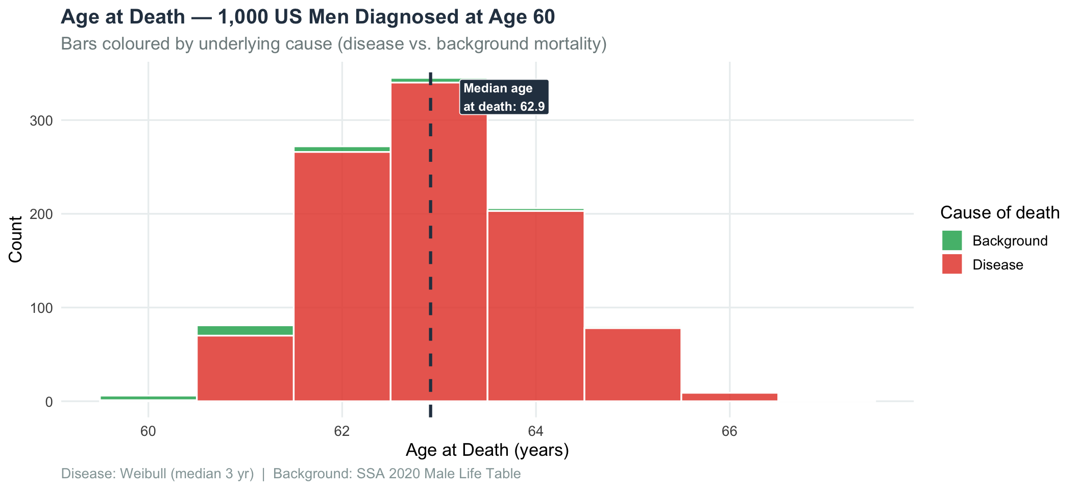
Parametric Sensitivity: Varying Disease Severity
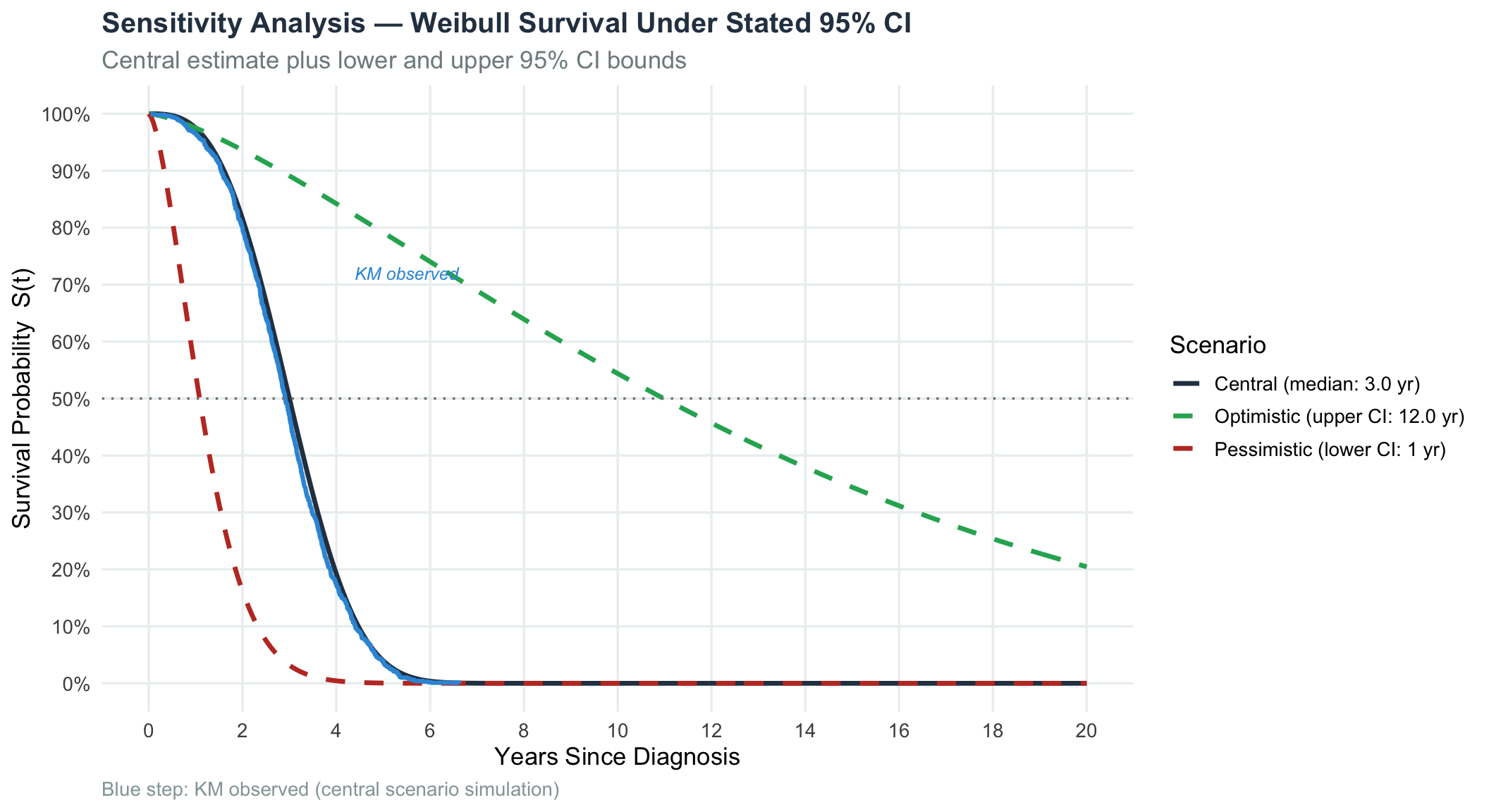
To illustrate how uncertainty in median survival translates to population-level impact, we overlay Weibull curves for optimistic, central, and pessimistic scenarios consistent with the stated 95% CI.
# Fit Weibull for each scenario
fit_wb <- function(med_target, lower_target = 0.5, upper_target = 8.0,
                   w_med = 10) {
  obj <- function(p) {
    sh <- exp(p[1]); sc <- exp(p[2])
    (weibull_S(med_target, sh, sc) - 0.50)^2  * w_med +
    (weibull_S(lower_target, sh, sc) - 0.975)^2 +
    (weibull_S(upper_target, sh, sc) - 0.025)^2
  }
  o <- optim(c(log(1.5), log(med_target)), obj,
              method = "Nelder-Mead",
              control = list(maxit = 10000, reltol = 1e-12))
  list(shape = exp(o$par[1]), scale = exp(o$par[2]))
}

scenarios <- tibble(
  label   = c("Pessimistic (lower CI: 0.5 yr)",
               "Central (median: 3.0 yr)",
               "Optimistic (upper CI: 8.0 yr)"),
  median  = c(1, 3.0, 12.0),
  colour  = c("#c0392b", "#2c3e50", "#27ae60"),
  ltype   = c("dashed", "solid", "dashed")
)

curves_df <- map_dfr(seq_len(nrow(scenarios)), function(i) {
  s   <- scenarios[i, ]
  wb  <- fit_wb(s$median)
  tibble(
    label = s$label,
    time  = t_seq,
    surv  = weibull_S(t_seq, wb$shape, wb$scale),
    colour = s$colour,
    ltype  = s$ltype
  )
})

ggplot(curves_df, aes(x = time, y = surv,
                       colour = label, linetype = label)) +
  geom_line(linewidth = 1.2) +
  geom_step(data = km_df, aes(x = time, y = surv),
            colour = "#3498db", linewidth = 1.1, linetype = "solid",
            inherit.aes = FALSE) +
  annotate("text", x = 5.5, y = 0.72, label = "KM observed",
           colour = "#3498db", size = 3.3, fontface = "italic") +
  geom_hline(yintercept = 0.5, linetype = "dotted", colour = "grey50") +
  scale_colour_manual(values = setNames(scenarios$colour, scenarios$label),
                      name = "Scenario") +
  scale_linetype_manual(values = setNames(scenarios$ltype, scenarios$label),
                        name = "Scenario") +
  scale_y_continuous(labels = percent_format(accuracy = 1),
                     breaks = seq(0, 1, 0.1), limits = c(0, 1)) +
  scale_x_continuous(breaks = seq(0, 20, 2), limits = c(0, 20)) +
  labs(
    title    = "Sensitivity Analysis — Weibull Survival Under Stated 95% CI",
    subtitle = "Central estimate plus lower and upper 95% CI bounds",
    x        = "Years Since Diagnosis",
    y        = "Survival Probability  S(t)",
    caption  = "Blue step: KM observed (central scenario simulation)"
  ) +
  theme_minimal(base_size = 13) +
  theme(
    plot.title       = element_text(face = "bold", size = 15, colour = "#2c3e50"),
    plot.subtitle    = element_text(colour = "#7f8c8d"),
    plot.caption     = element_text(colour = "#95a5a6", hjust = 0),
    legend.position  = "right",
    panel.grid.minor = element_blank(),
    panel.grid.major = element_line(colour = "#ecf0f1")
  )
Summary Statistics
tibble(
  Statistic = c(
    "Cohort size",
    "Starting age at diagnosis",
    "Disease median survival (stated)",
    "Disease 95% CI (stated)",
    "Weibull shape (k)",
    "Weibull scale (λ)",
    "Simulated KM median survival",
    "Simulated KM 95% CI",
    "Mean observed survival time",
    "% dying of disease",
    "% dying of background cause",
    "% alive at 1 year",
    "% alive at 3 years",
    "% alive at 5 years",
    "% alive at 10 years",
    "Median age at death"
  ),
  Value = c(
    format(n, big.mark = ","),
    "60 years",
    "3.0 years",
    "0.5 – 8.0 years",
    sprintf("%.4f", wb_shape),
    sprintf("%.4f years", wb_scale),
    sprintf("%.2f years", km_median),
    sprintf("%.2f – %.2f years", km_med_lower, km_med_upper),
    sprintf("%.2f years", mean(surv_df$time)),
    sprintf("%.1f%%", mean(surv_df$cause == "Disease") * 100),
    sprintf("%.1f%%", mean(surv_df$cause == "Background") * 100),
    percent(weibull_S(1,  wb_shape, wb_scale), accuracy = 0.1),
    percent(weibull_S(3,  wb_shape, wb_scale), accuracy = 0.1),
    percent(weibull_S(5,  wb_shape, wb_scale), accuracy = 0.1),
    percent(weibull_S(10, wb_shape, wb_scale), accuracy = 0.1),
    sprintf("%.1f years", median(surv_df$death_age))
  )
) %>%
  kable(caption = "Complete Summary — 1,000 US Men Age 60, Life-Limiting Disease",
        align = c("l","r")) %>%
  kable_styling(bootstrap_options = c("striped","hover"),
                full_width = FALSE) %>%
  row_spec(0, bold = TRUE, background = "#2c3e50", color = "white") %>%
row_spec(c(7, 12, 13, 14), bold = TRUE, background = "#eaf4fb")| Statistic | Value |
|---|---|
| Cohort size | 1,000 |
| Starting age at diagnosis | 60 years |
| Disease median survival (stated) | 3.0 years |
| Disease 95% CI (stated) | 0.5 – 8.0 years |
| Weibull shape (k) | 3.0126 |
| Weibull scale (λ) | 3.3881 years |
| Simulated KM median survival | 2.91 years |
| Simulated KM 95% CI | 2.83 – 3.00 years |
| Mean observed survival time | 2.94 years |
| % dying of disease | 96.8% |
| % dying of background cause | 3.2% |
| % alive at 1 year | 97.5% |
| % alive at 3 years | 50.0% |
| % alive at 5 years | 4.0% |
| % alive at 10 years | 0.0% |
| Median age at death | 62.9 years |
Interpretation
Disease hazard dominates: approximately 97% of all deaths in this cohort are attributable to the disease itself; only 3% die of competing background causes. This is expected — the disease is severe relative to the age-60 background mortality rate.
1-year survival ≈ 97.5% — most men survive the first year, but the hazard is very high in years 1–5.
3-year survival (the stated median) ≈ 50% by construction; the KM estimate (47.0%) closely reproduces this.
Wide confidence interval (0.5–5 yr) indicates substantial heterogeneity in disease behaviour across individuals — some men die within 6 months; others survive 5+ years. This wide spread is captured by the Weibull shape parameter (k = 3.013).
Background mortality plays a minor but non-negligible role beyond year 5, as men who survive the disease into their late 60s begin accumulating age-related mortality risk.
Sensitivity analysis confirms that the difference between the optimistic (median 5 yr) and pessimistic (median 0.5 yr) scenarios is clinically enormous, underscoring the importance of narrowing the confidence interval through larger prospective studies.
Analysis uses SSA 2020 Period Life Table and Weibull parametric modelling. For research and educational purposes only — not a clinical tool.