
Monte Carlo estimate of 𝛑
An elegant way to demonstrate the Monte Carlo technique is by estimating \(\pi\) in a simple geometry problem. Given a circle of radius r inscribed in a square of side 2r, the area of the circle is \(\pi*r^2\) and the area of the square is \(4r^2\). The ratio of those areas is \(\pi /4\), so if you scatter points randomly and uniformly, the fraction landing inside the circle will also converge to \(\pi/4\).
The Monte Carlo name was coined by the mathematician Stanislaw Ulam during his work on the Manhattan Project. He realized that some physics problems are unsolvable or too complex for direct calculation but can be approximated by running many random simulations. The circle-in-a-square problem became the go-to teaching example of the technique because it’s so easy to visualize and verify.
Estimate \(\pi\) once
n <- 10000
x_rand <- runif(n, min = -r, max = r)
y_rand <- runif(n, min = -r, max = r)
distance_from_center <- sqrt(x_rand^2 + y_rand^2)
is_inside <- distance_from_center <= r
point_df <- data.frame(x = x_rand, y = y_rand, distance_from_center, is_inside)
 summary(point_df$is_inside)
## Mode FALSE TRUE
## logical 2181 7819# Count TRUEs
# num_inside <- sum(point_df$is_inside)
pi_hat <- 4 * sum(point_df$is_inside)/n; pi_hat## [1] 3.1276Make a function to estimate
pi_est <- function(n) {
  x_rand <- runif(n, min = -r, max = r)
  y_rand <- runif(n, min = -r, max = r)
  distance_from_center <- sqrt(x_rand^2 + y_rand^2)
  is_inside <- distance_from_center <= r
  point_df <- data.frame(x = x_rand, y = y_rand, distance_from_center, is_inside)
  pi_hat <- 4 * ( sum(point_df$is_inside)/n)
  return(pi_hat)
}
pi_est(1000)
## [1] 3.172Generic Monte Carlo Simulation + Median + CI Plot
# Example: Estimate π using n random points
fn <- function(n) {
  x <- runif(n, -1, 1)
  y <- runif(n, -1, 1)
  inside <- (x^2 + y^2) <= 1
  pi_estimate <- 4 * mean(inside)
  return(pi_estimate)
}

sample_sizes <- seq(500, 10000, by = 100)   # from 500 to 10,000
n_replications <- 500                       # Number of times to run each sample size
set.seed(11)

# This part is the Monte Carlo simulation
results <- tibble(sample_size = sample_sizes) %>%
  mutate(
    estimates = map(sample_size, function(n) {
      replicate(n_replications, fn(n))
    })
  ) %>%
  mutate(
    median = map_dbl(estimates, median),
    lower_ci = map_dbl(estimates, ~ quantile(.x, 0.025)),
    upper_ci = map_dbl(estimates, ~ quantile(.x, 0.975))
  )

tt <- tibble(id=seq(1:100)) %>%
  mutate(
    rep_no = runif(100,0,1)
  )
#?mutate
4. Plot: Median + 95% Confidence Intervals
g <- ggplot(results, aes(x = sample_size)) +
  #geom_ribbon(aes(ymin = lower_ci, ymax = upper_ci),
  #            fill = "steelblue", alpha = 0.15) +
  geom_line(aes(y = median), color = "steelblue", linewidth = 1.2) +
  geom_smooth(aes(y=upper_ci), method='loess', color ="darkgray", linewidth = 0.8) +
  geom_smooth(aes(y=lower_ci), method='loess', color ="darkgray", linewidth = 0.8) +
  #geom_point(aes(y=upper_ci), color ="darkgray", size = 0.4) +
  #geom_point(aes(y=lower_ci), color ="darkgray", size = 0.4) +
  geom_ribbon(aes(ymin = lower_ci, ymax = upper_ci), color = "lightblue", alpha = 0.1)+
  geom_hline(yintercept = pi, color = "red", linewidth = 0.3) +
  scale_x_continuous( breaks=seq(0,10000,1000)) +
  labs(title = "Monte Carlo Simulation: Convergence of π Estimate",
       subtitle = paste("Median of", n_replications, "replications per sample size"),
       x = "Sample Size (n)",
       y = "Estimated π") +
  annotate("text", x = max(sample_sizes)*0.75, y = pi + 0.015,
           label = "True π ≈ 3.141592", color = "red", size = 4.5) +
  #theme_minimal(base_size = 14) +
  theme(plot.title = element_text(face = "bold")); g #, hjust = 0.5
## `geom_smooth()` using formula = 'y ~ x'
## `geom_smooth()` using formula = 'y ~ x'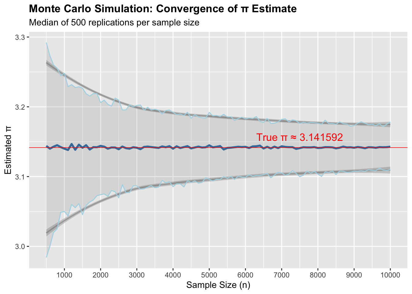
# Show summary table

print(results %>% select(sample_size, median, lower_ci, upper_ci), n = 100)
## # A tibble: 96 × 4
## sample_size median lower_ci upper_ci
## <dbl> <dbl> <dbl> <dbl>
## 1 500 3.14 2.98 3.29
## 2 600 3.14 3 3.27
## 3 700 3.14 3.02 3.26
## 4 800 3.14 3.02 3.26
## 5 900 3.14 3.05 3.24
## 6 1000 3.14 3.05 3.25
## 7 1100 3.14 3.04 3.23
## 8 1200 3.15 3.06 3.23
## 9 1300 3.14 3.06 3.23
## 10 1400 3.15 3.06 3.23
## 11 1500 3.14 3.05 3.23
## 12 1600 3.14 3.06 3.22
## 13 1700 3.14 3.06 3.22
## 14 1800 3.14 3.07 3.22
## 15 1900 3.14 3.07 3.22
## 16 2000 3.14 3.07 3.21
## 17 2100 3.14 3.08 3.21
## 18 2200 3.14 3.07 3.20
## 19 2300 3.14 3.08 3.20
## 20 2400 3.14 3.08 3.21
## 21 2500 3.14 3.07 3.21
## 22 2600 3.14 3.09 3.20
## 23 2700 3.14 3.08 3.20
## 24 2800 3.14 3.08 3.20
## 25 2900 3.14 3.09 3.2
## 26 3000 3.14 3.09 3.20
## 27 3100 3.14 3.08 3.20
## 28 3200 3.14 3.08 3.20
## 29 3300 3.14 3.08 3.20
## 30 3400 3.14 3.09 3.20
## 31 3500 3.14 3.08 3.20
## 32 3600 3.14 3.08 3.20
## 33 3700 3.14 3.09 3.19
## 34 3800 3.14 3.09 3.19
## 35 3900 3.14 3.09 3.20
## 36 4000 3.14 3.09 3.19
## 37 4100 3.14 3.09 3.19
## 38 4200 3.14 3.09 3.19
## 39 4300 3.14 3.09 3.19
## 40 4400 3.14 3.09 3.19
## 41 4500 3.14 3.09 3.18
## 42 4600 3.14 3.09 3.19
## 43 4700 3.14 3.09 3.19
## 44 4800 3.14 3.09 3.18
## 45 4900 3.14 3.10 3.18
## 46 5000 3.14 3.10 3.19
## 47 5100 3.14 3.09 3.19
## 48 5200 3.14 3.10 3.19
## 49 5300 3.14 3.10 3.19
## 50 5400 3.14 3.1 3.19
## 51 5500 3.14 3.10 3.19
## 52 5600 3.14 3.10 3.19
## 53 5700 3.14 3.10 3.18
## 54 5800 3.14 3.10 3.18
## 55 5900 3.14 3.10 3.19
## 56 6000 3.14 3.10 3.18
## 57 6100 3.14 3.10 3.18
## 58 6200 3.14 3.10 3.18
## 59 6300 3.14 3.10 3.19
## 60 6400 3.14 3.10 3.18
## 61 6500 3.14 3.10 3.18
## 62 6600 3.14 3.10 3.18
## 63 6700 3.14 3.10 3.18
## 64 6800 3.14 3.10 3.18
## 65 6900 3.14 3.11 3.18
## 66 7000 3.14 3.11 3.18
## 67 7100 3.14 3.10 3.18
## 68 7200 3.14 3.10 3.18
## 69 7300 3.14 3.11 3.18
## 70 7400 3.14 3.10 3.18
## 71 7500 3.14 3.10 3.18
## 72 7600 3.14 3.10 3.18
## 73 7700 3.14 3.11 3.18
## 74 7800 3.14 3.10 3.18
## 75 7900 3.14 3.11 3.18
## 76 8000 3.14 3.10 3.18
## 77 8100 3.14 3.10 3.17
## 78 8200 3.14 3.11 3.18
## 79 8300 3.14 3.11 3.18
## 80 8400 3.14 3.11 3.18
## 81 8500 3.14 3.10 3.17
## 82 8600 3.14 3.11 3.18
## 83 8700 3.14 3.11 3.18
## 84 8800 3.14 3.11 3.18
## 85 8900 3.14 3.11 3.17
## 86 9000 3.14 3.11 3.17
## 87 9100 3.14 3.11 3.18
## 88 9200 3.14 3.11 3.18
## 89 9300 3.14 3.11 3.18
## 90 9400 3.14 3.11 3.17
## 91 9500 3.14 3.11 3.17
## 92 9600 3.14 3.11 3.17
## 93 9700 3.14 3.11 3.18
## 94 9800 3.14 3.11 3.17
## 95 9900 3.14 3.11 3.17
## 96 10000 3.14 3.11 3.18