
Understanding the Weibull Distribution
1. Introduction
The Weibull distribution is one of the most widely used distributions in reliability engineering, survival analysis, and failure-time modelling. Named after Swedish engineer Waloddi Weibull (1951), it is prized for its flexibility: by tuning just two parameters it can mimic an exponential, a normal-like bell, or a heavily skewed shape.
Why use the Weibull?
- Models time-to-failure of mechanical and electronic components
- Widely used in survival analysis (time-to-event data)
- Flexible enough to model early failures (infant mortality), random failures, or wear-out failures
- Foundation of accelerated life testing and warranty analysis
2. Mathematical Definition
2.1 Probability Density Function (PDF)
The two-parameter Weibull PDF is:
\[f(x; k, \lambda) = \frac{k}{\lambda} \left(\frac{x}{\lambda}\right)^{k-1} e^{-(x/\lambda)^k}, \quad x \geq 0\]
where:
| Parameter | Symbol | Role |
|---|---|---|
| Shape | \(k > 0\) | Controls the shape of the distribution |
| Scale | \(\lambda > 0\) | Stretches or compresses the distribution along the x-axis |
2.2 Cumulative Distribution Function (CDF)
\[F(x; k, \lambda) = 1 - e^{-(x/\lambda)^k}\]
2.3 Survival (Reliability) Function
\[S(x) = 1 - F(x) = e^{-(x/\lambda)^k}\]
2.4 Hazard Function
The hazard function (instantaneous failure rate) is:
\[h(x) = \frac{f(x)}{S(x)} = \frac{k}{\lambda}\left(\frac{x}{\lambda}\right)^{k-1}\]
This is one of the Weibull’s most powerful features — the shape of the hazard is entirely determined by \(k\).
3. The Role of Shape Parameter \(k\)
library(ggplot2)
library(dplyr)
library(tidyr)

# Define a grid of x values and shape parameters to compare
x     <- seq(0.01, 4, length.out = 500)
k_vals <- c(0.5, 1, 1.5, 2, 3.5)
lambda <- 1  # fix scale = 1 for clarity

pdf_data <- lapply(k_vals, function(k) {
  data.frame(
    x   = x,
    pdf = dweibull(x, shape = k, scale = lambda),
    k   = paste0("k = ", k)
  )
}) |> bind_rows()

ggplot(pdf_data, aes(x = x, y = pdf, color = k)) +
  geom_line(linewidth = 1.1) +
  labs(
    title    = "Weibull PDF for Different Shape Parameters (λ = 1)",
    x        = "x",
    y        = "Density f(x)",
    color    = "Shape k"
  ) +
  theme_minimal(base_size = 13) +
  coord_cartesian(ylim = c(0, 2))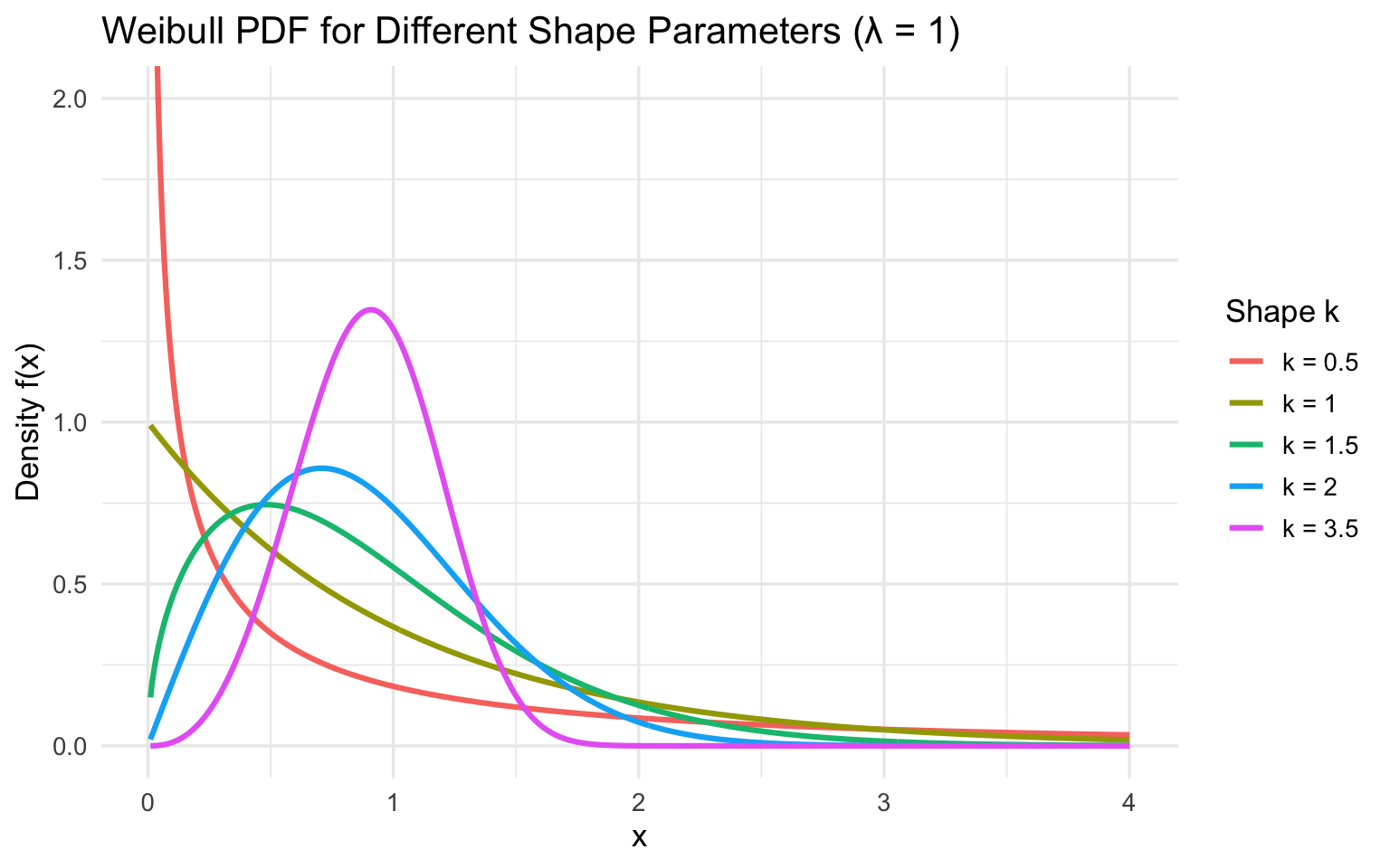
Interpreting \(k\)
| \(k\) value | Hazard shape | Real-world meaning |
|---|---|---|
| \(k < 1\) | Decreasing hazard | Infant mortality — failures most likely early |
| \(k = 1\) | Constant hazard | Random failures — reduces to Exponential |
| \(k \approx 2.5\) | Increasing hazard | Approximates a Normal distribution |
| \(k > 1\) | Increasing hazard | Wear-out failures — risk grows with age |
4. The Role of Scale Parameter \(\lambda\)
lambda_vals <- c(0.5, 1, 2, 3)
k_fixed     <- 2  # fix shape = 2

scale_data <- lapply(lambda_vals, function(lam) {
  data.frame(
    x      = x,
    pdf    = dweibull(x, shape = k_fixed, scale = lam),
    lambda = paste0("λ = ", lam)
  )
}) |> bind_rows()

ggplot(scale_data, aes(x = x, y = pdf, color = lambda)) +
  geom_line(linewidth = 1.1) +
  labs(
    title = "Weibull PDF for Different Scale Parameters (k = 2)",
    x     = "x",
    y     = "Density f(x)",
    color = "Scale λ"
  ) +
  theme_minimal(base_size = 13)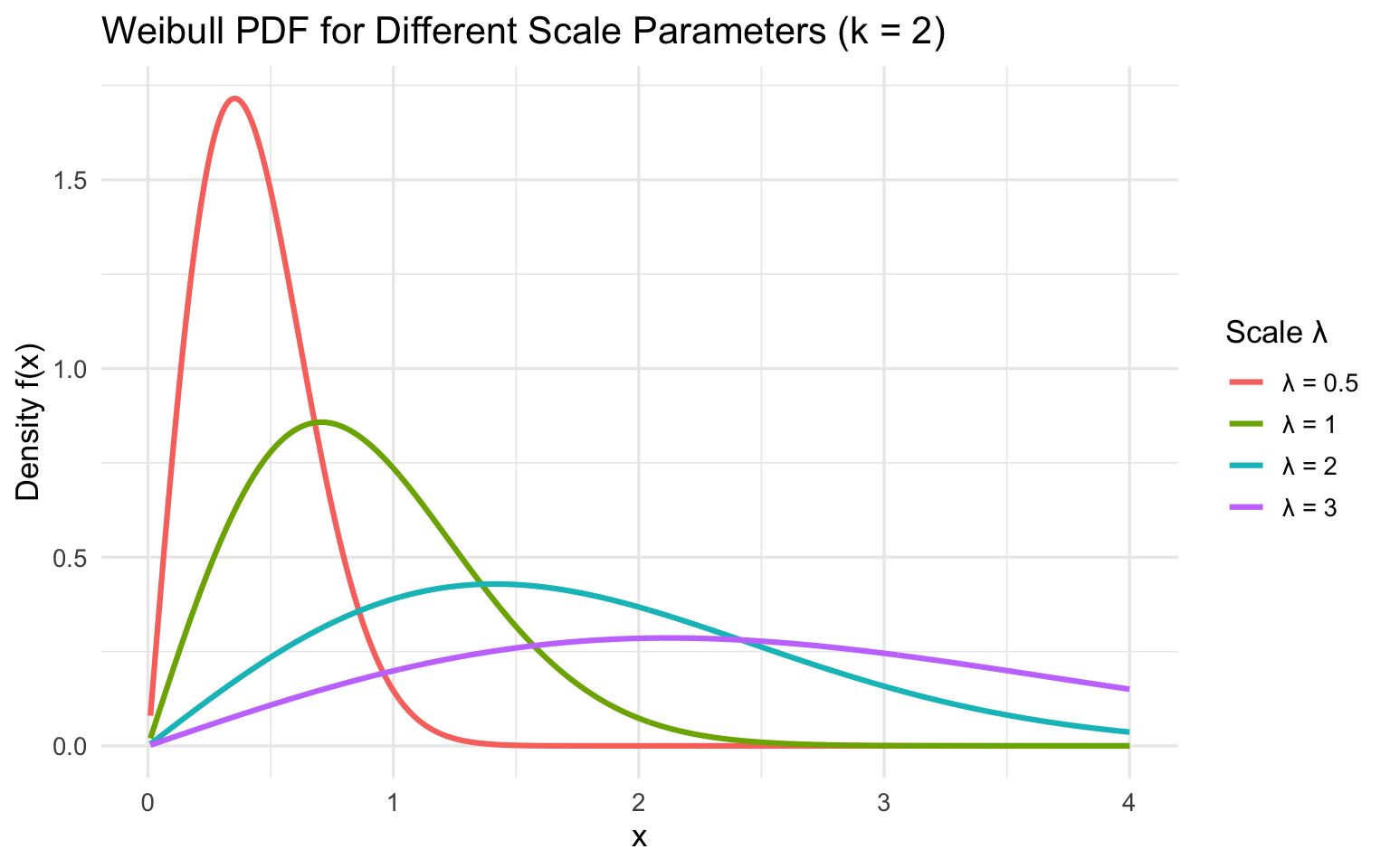
Key insight: \(\lambda\) is the characteristic life — the value of \(x\) at which \(F(x) \approx 63.2\%\) of items have failed, regardless of \(k\).
5. R Functions for the Weibull
R provides four built-in functions for the Weibull distribution:
# Parameters
k   <- 2      # shape
lam <- 3      # scale

# --- dweibull: probability density at x = 2 ---
d_val <- dweibull(x = 2, shape = k, scale = lam)
cat("PDF at x=2:      ", round(d_val, 5), "\n")
## PDF at x=2: 0.28497# --- pweibull: cumulative probability P(X <= 2) ---
p_val <- pweibull(q = 2, shape = k, scale = lam)
cat("P(X <= 2): ", round(p_val, 5), "\n")## P(X <= 2): 0.35882# --- qweibull: quantile (inverse CDF) — 50th percentile ---
q_val <- qweibull(p = 0.5, shape = k, scale = lam)
cat("Median (50th %): ", round(q_val, 5), "\n")## Median (50th %): 2.49766# --- rweibull: random samples ---
set.seed(42)
samples <- rweibull(n = 1000, shape = k, scale = lam)
cat("Sample mean: ", round(mean(samples), 5), "\n")## Sample mean: 2.7224cat("Sample SD: ", round(sd(samples), 5), "\n")## Sample SD: 1.429546. Key Summary Statistics
For a Weibull(\(k\), \(\lambda\)) random variable \(X\):
| Statistic | Formula |
|---|---|
| Mean | \(\lambda \, \Gamma\!\left(1 + \frac{1}{k}\right)\) |
| Variance | \(\lambda^2 \left[\Gamma\!\left(1 + \frac{2}{k}\right) - \left(\Gamma\!\left(1 + \frac{1}{k}\right)\right)^2\right]\) |
| Median | \(\lambda (\ln 2)^{1/k}\) |
| Mode (k>1) | \(\lambda \left(\frac{k-1}{k}\right)^{1/k}\) |
weibull_stats <- function(k, lambda) {
  mean_val   <- lambda * gamma(1 + 1/k)
  var_val    <- lambda^2 * (gamma(1 + 2/k) - (gamma(1 + 1/k))^2)
  median_val <- lambda * (log(2))^(1/k)
  mode_val   <- if (k > 1) lambda * ((k - 1) / k)^(1/k) else 0

  cat(sprintf("Weibull(k=%.1f, λ=%.1f)\n", k, lambda))
  cat(sprintf("  Mean:   %.4f\n", mean_val))
  cat(sprintf("  SD:     %.4f\n", sqrt(var_val)))
  cat(sprintf("  Median: %.4f\n", median_val))
  cat(sprintf("  Mode:   %.4f\n\n", mode_val))
}

weibull_stats(0.5, 1)
## Weibull(k=0.5, λ=1.0)
## Mean: 2.0000
## SD: 4.4721
## Median: 0.4805
## Mode: 0.0000weibull_stats(1.0, 1)## Weibull(k=1.0, λ=1.0)
## Mean: 1.0000
## SD: 1.0000
## Median: 0.6931
## Mode: 0.0000weibull_stats(2.0, 1)## Weibull(k=2.0, λ=1.0)
## Mean: 0.8862
## SD: 0.4633
## Median: 0.8326
## Mode: 0.7071weibull_stats(3.5, 1)## Weibull(k=3.5, λ=1.0)
## Mean: 0.8997
## SD: 0.2847
## Median: 0.9006
## Mode: 0.90837. Hazard Functions Visualised
The hazard function is critical in reliability — it tells us how the instantaneous risk of failure changes over time.
hazard_data <- lapply(k_vals, function(k) {
  h <- dweibull(x, shape = k, scale = 1) / pweibull(x, shape = k, scale = 1, lower.tail = FALSE)
  data.frame(x = x, hazard = h, k = paste0("k = ", k))
}) |> bind_rows()

ggplot(hazard_data, aes(x = x, y = hazard, color = k)) +
  geom_line(linewidth = 1.1) +
  coord_cartesian(ylim = c(0, 5)) +
  labs(
    title  = "Weibull Hazard Function h(x) for Different Shape Values (λ = 1)",
    x      = "Time x",
    y      = "Hazard h(x)",
    color  = "Shape k"
  ) +
  theme_minimal(base_size = 13)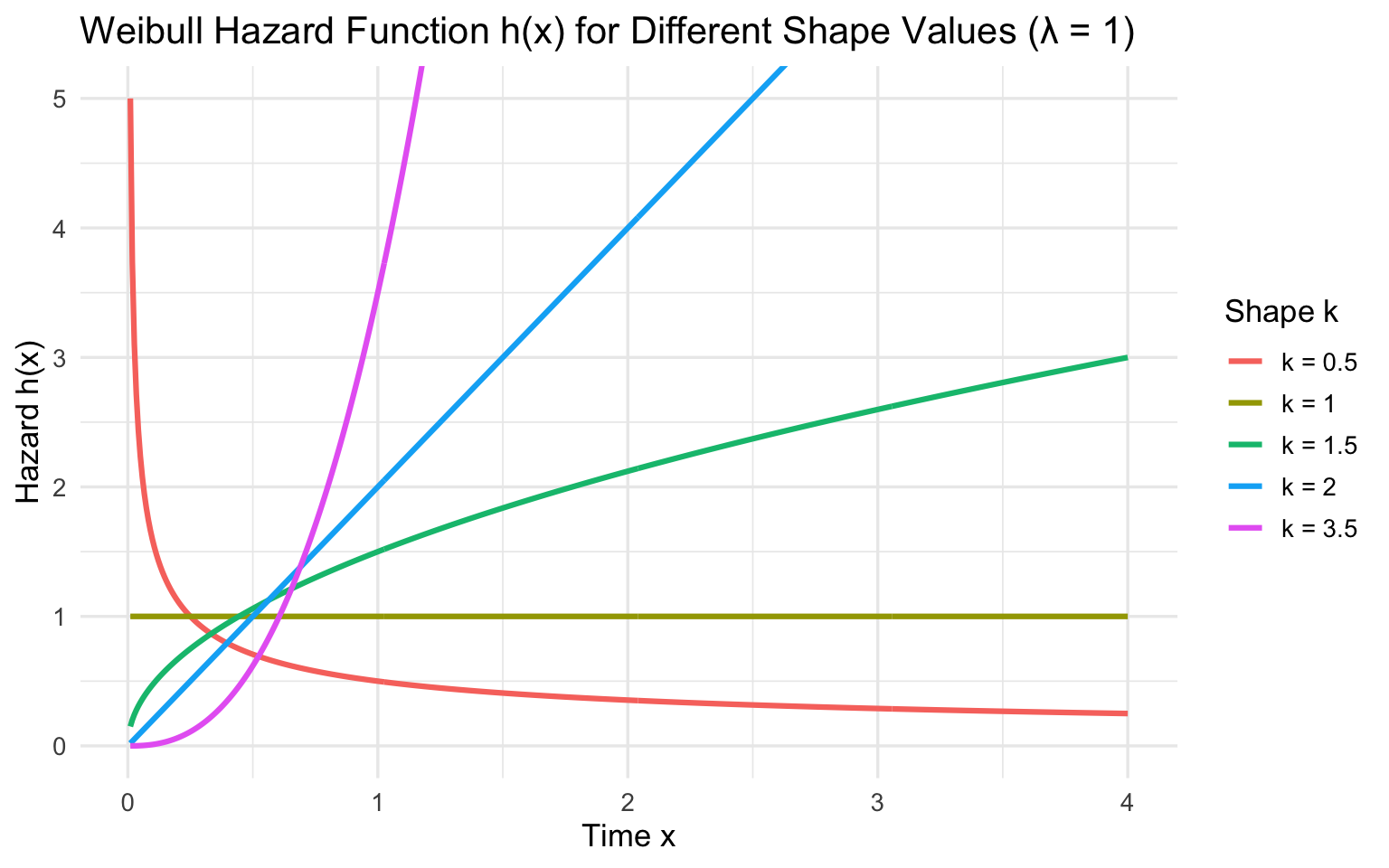
8. Fitting a Weibull Distribution to Data
8.1 Simulate Data
set.seed(123)
true_k   <- 2.5
true_lam <- 4.0

failure_times <- rweibull(n = 200, shape = true_k, scale = true_lam)
summary(failure_times)
## Min. 1st Qu. Median Mean 3rd Qu. Max.
## 0.508 2.504 3.526 3.484 4.445 8.8978.2 MLE Estimation with MASS::fitdistr
library(MASS)

fit <- fitdistr(failure_times, densfun = "weibull")
print(fit)
## shape scale
## 2.6844687 3.9167731
## (0.1464182) (0.1085882)cat("\nTrue parameters: k =", true_k, " λ =", true_lam, "\n")##
## True parameters: k = 2.5 λ = 4cat("Estimated: k =", round(fit$estimate["shape"], 3),
" λ =", round(fit$estimate["scale"], 3), "\n")## Estimated: k = 2.684 λ = 3.9178.3 Goodness-of-Fit: Density Overlay
k_hat   <- fit$estimate["shape"]
lam_hat <- fit$estimate["scale"]

ggplot(data.frame(x = failure_times), aes(x = x)) +
  geom_histogram(aes(y = after_stat(density)), bins = 25,
                 fill = "#4E9AF1", color = "white", alpha = 0.7) +
  stat_function(fun = dweibull, args = list(shape = k_hat, scale = lam_hat),
                color = "#E63946", linewidth = 1.3, linetype = "solid") +
  stat_function(fun = dweibull, args = list(shape = true_k, scale = true_lam),
                color = "#2A9D8F", linewidth = 1.1, linetype = "dashed") +
  labs(
    title    = "Fitted Weibull vs True Distribution",
    subtitle = "Red = fitted MLE | Green dashed = true distribution",
    x        = "Failure Time",
    y        = "Density"
  ) +
  theme_minimal(base_size = 13)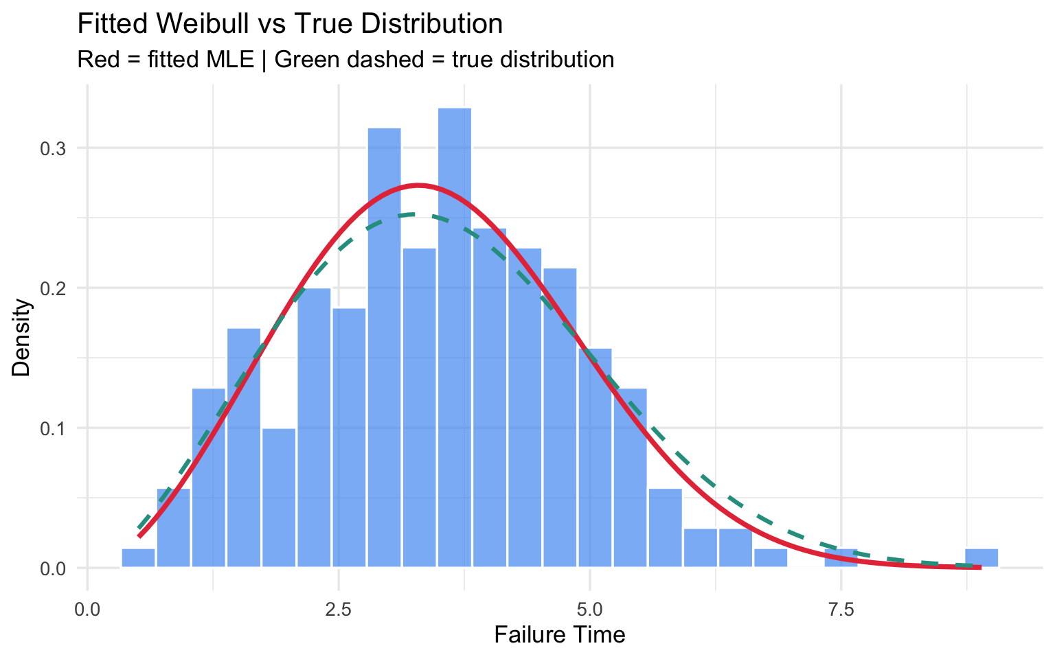
8.4 Q-Q Plot
# Compute theoretical quantiles under fitted model
probs     <- ppoints(length(failure_times))
theor_q   <- qweibull(probs, shape = k_hat, scale = lam_hat)
observed_q <- sort(failure_times)

ggplot(data.frame(theoretical = theor_q, observed = observed_q),
       aes(x = theoretical, y = observed)) +
  geom_point(alpha = 0.5, color = "#4E9AF1") +
  geom_abline(slope = 1, intercept = 0, color = "#E63946", linewidth = 1) +
  labs(
    title = "Weibull Q-Q Plot",
    x     = "Theoretical Quantiles",
    y     = "Sample Quantiles"
  ) +
  theme_minimal(base_size = 13)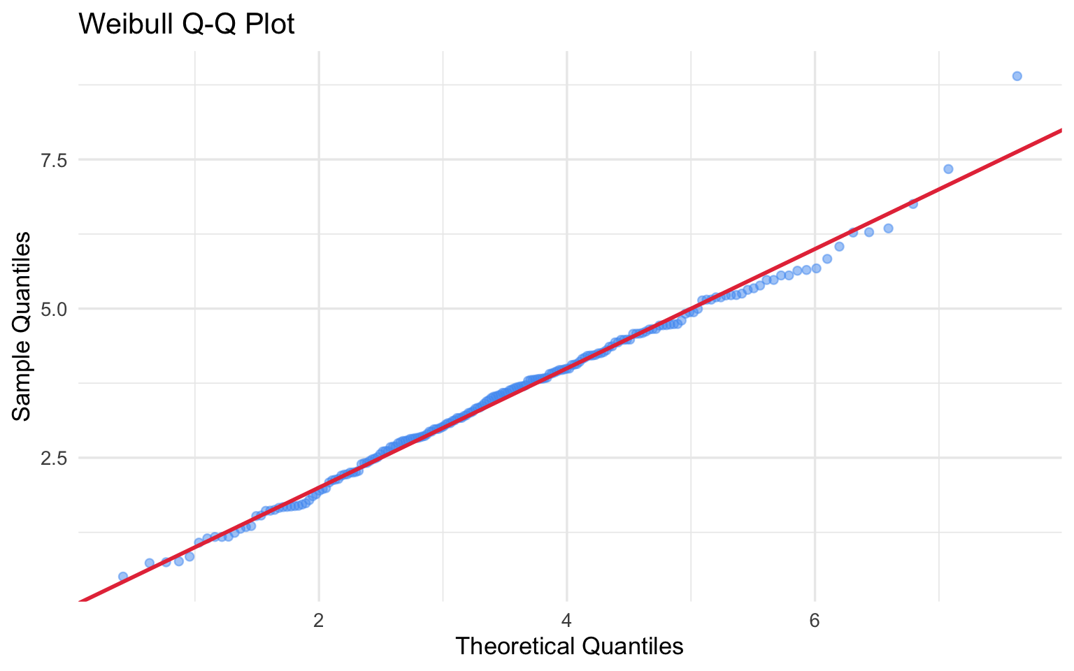
Points close to the red line indicate a good Weibull fit.
9. Real-World Example: Bearing Failures
A factory records the operating hours until 50 ball bearings fail. We model these using the Weibull distribution.
set.seed(99)
# Simulate bearing lifetimes (hours)
bearing_hours <- rweibull(50, shape = 3, scale = 2000)

# Fit
bearing_fit <- fitdistr(bearing_hours, "weibull")
k_b   <- bearing_fit$estimate["shape"]
lam_b <- bearing_fit$estimate["scale"]

cat("Estimated shape (k):  ", round(k_b, 3), "\n")
## Estimated shape (k): 2.883cat("Estimated scale (λ): ", round(lam_b, 3), "\n\n")## Estimated scale (λ): 2070.18# Probability of failure before 1500 hours
p_fail_1500 <- pweibull(1500, shape = k_b, scale = lam_b)
cat(sprintf("P(failure before 1500 hrs) = %.1f%%\n", p_fail_1500 * 100))## P(failure before 1500 hrs) = 32.6%# B10 life — time at which 10% of bearings have failed
b10 <- qweibull(0.10, shape = k_b, scale = lam_b)
cat(sprintf("B10 life (10%% fail): %.0f hours\n", b10))## B10 life (10% fail): 948 hours# Mean time to failure
mttf <- lam_b * gamma(1 + 1/k_b)
cat(sprintf("Mean Time to Failure (MTTF): %.0f hours\n", mttf))## Mean Time to Failure (MTTF): 1846 hourst_seq <- seq(0, 4000, length.out = 300)
surv <- pweibull(t_seq, shape = k_b, scale = lam_b, lower.tail = FALSE)
ggplot(data.frame(t = t_seq, S = surv), aes(x = t, y = S)) +
geom_line(color = "#2A9D8F", linewidth = 1.3) +
geom_hline(yintercept = 0.90, linetype = "dashed", color = "#E63946") +
geom_vline(xintercept = b10, linetype = "dashed", color = "#E63946") +
annotate("text", x = b10 + 100, y = 0.95,
label = paste0("B10 = ", round(b10, 0), " hrs"), hjust = 0) +
labs(
title = "Bearing Survival (Reliability) Curve",
x = "Operating Hours",
y = "Survival Probability S(t)"
) +
scale_y_continuous(labels = scales::percent) +
theme_minimal(base_size = 13)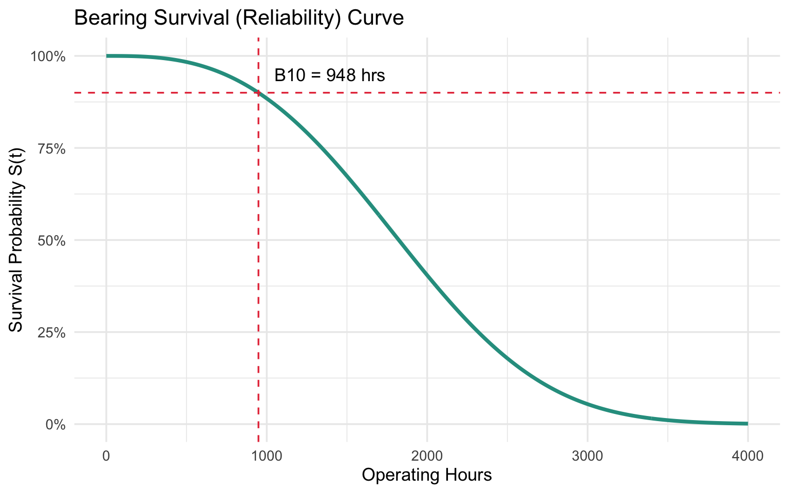
10. Connections to Other Distributions
| Special case | Parameters | Equivalent distribution |
|---|---|---|
| \(k = 1\) | Any \(\lambda\) | Exponential(\(1/\lambda\)) |
| \(k = 2\) | Any \(\lambda\) | Rayleigh distribution |
| \(k \approx 3.6\) | Any \(\lambda\) | Approximately Normal |
| \(k = 1, \lambda = 1\) | — | Standard Exponential |
x2 <- seq(0.001, 5, length.out = 500)

special <- bind_rows(
  data.frame(x = x2,
             y = dweibull(x2, shape = 1, scale = 1),
             dist = "Weibull(k=1) = Exponential"),
  data.frame(x = x2,
             y = dweibull(x2, shape = 2, scale = 1),
             dist = "Weibull(k=2) = Rayleigh"),
  data.frame(x = x2,
             y = dweibull(x2, shape = 3.6, scale = 1),
             dist = "Weibull(k=3.6) ≈ Normal")
)

ggplot(special, aes(x = x, y = y, color = dist)) +
  geom_line(linewidth = 1.2) +
  labs(title = "Weibull Special Cases", x = "x", y = "Density", color = NULL) +
  theme_minimal(base_size = 13) +
  theme(legend.position = "top")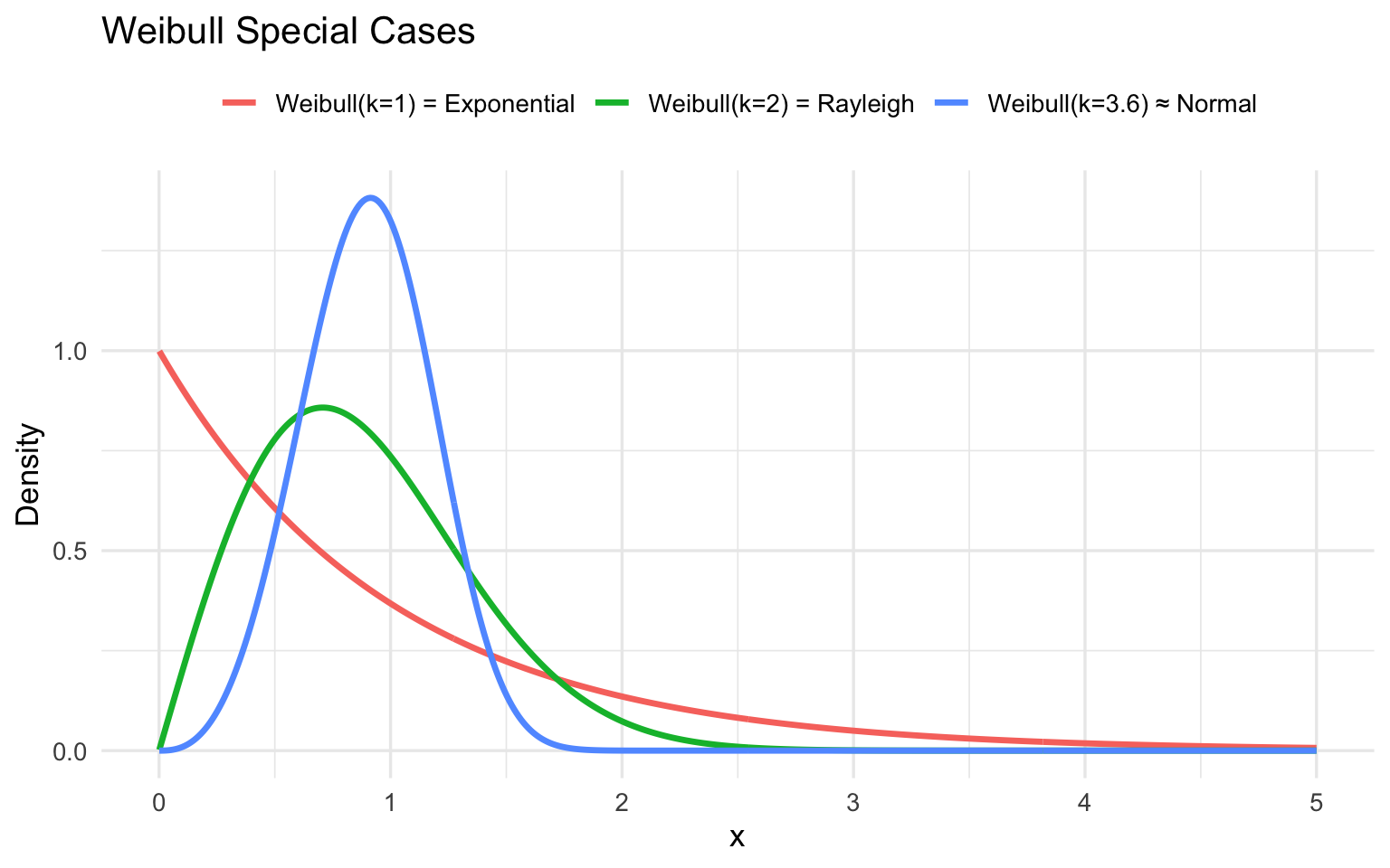
11. Summary
| Topic | Key Points |
|---|---|
| Shape \(k\) | \(k<1\): decreasing hazard; \(k=1\): constant; \(k>1\): increasing hazard |
| Scale \(\lambda\) | Characteristic life; 63.2% of items failed at \(x = \lambda\) |
| Flexibility | Encompasses Exponential, Rayleigh, and near-Normal as special cases |
| R functions | dweibull, pweibull, qweibull,
rweibull, MASS::fitdistr |
| Applications | Reliability, survival analysis, warranty, accelerated life testing |
Session Info
sessionInfo()## R version 4.5.3 (2026-03-11)
## Platform: aarch64-apple-darwin20
## Running under: macOS Tahoe 26.4.1
##
## Matrix products: default
## BLAS: /Library/Frameworks/R.framework/Versions/4.5-arm64/Resources/lib/libRblas.0.dylib
## LAPACK: /Library/Frameworks/R.framework/Versions/4.5-arm64/Resources/lib/libRlapack.dylib; LAPACK version 3.12.1
##
## locale:
## [1] en_US.UTF-8/en_US.UTF-8/en_US.UTF-8/C/en_US.UTF-8/en_US.UTF-8
##
## time zone: America/Phoenix
## tzcode source: internal
##
## attached base packages:
## [1] stats graphics grDevices utils datasets methods base
##
## other attached packages:
## [1] MASS_7.3-65 tidyr_1.3.2 dplyr_1.2.1 ggplot2_4.0.2
##
## loaded via a namespace (and not attached):
## [1] vctrs_0.7.1 cli_3.6.5 knitr_1.51 rlang_1.1.7
## [5] xfun_0.56 purrr_1.2.1 generics_0.1.4 S7_0.2.1
## [9] jsonlite_2.0.0 labeling_0.4.3 glue_1.8.0 htmltools_0.5.9
## [13] sass_0.4.10 scales_1.4.0 rmarkdown_2.30 grid_4.5.3
## [17] tibble_3.3.1 evaluate_1.0.5 jquerylib_0.1.4 fastmap_1.2.0
## [21] yaml_2.3.12 lifecycle_1.0.5 compiler_4.5.3 RColorBrewer_1.1-3
## [25] pkgconfig_2.0.3 rstudioapi_0.18.0 farver_2.1.2 digest_0.6.39
## [29] R6_2.6.1 tidyselect_1.2.1 pillar_1.11.1 magrittr_2.0.4
## [33] bslib_0.10.0 withr_3.0.2 tools_4.5.3 gtable_0.3.6
## [37] cachem_1.1.0