
Effect Sizes and Cohen's d in Biomedical Research
Contents
- Introduction
- What is Cohen’s d?
- Visualising Cohen’s d
- Why Context Beats Benchmarks in Biomedical Research
- Variants and Corrections
- MCID: The Clinical Alternative to Cohen’s Benchmarks
- R Toolkit
- Summary
1. Introduction
A p-value answers one question: how surprised should I be if the null hypothesis were true? It says nothing about whether the effect matters clinically. A trial of 50,000 patients can return p < 0.0001 for a drug that lowers blood pressure by 0.3 mmHg — a difference invisible to any clinician and irrelevant to any patient.
Effect sizes express the magnitude of an effect, independent of sample size. Cohen’s d is the most widely reported effect size in medicine, yet it is also one of the most consistently misread metrics in the literature. Cohen’s own labels — “small” (d = 0.2), “medium” (d = 0.5), “large” (d = 0.8) — were calibrated against 1950s–1960s behavioural science, not against any biomedical outcome. Applying them uncritically to clinical data produces absurd conclusions: that statins are “small” (they are; they also prevent millions of deaths annually) and that a poorly-designed diet intervention is “large” (it might be; it might also harm compliance and be unmeasurable in the real world).
This post works through what Cohen’s d means, shows it visually, maps it to clinically interpretable metrics, and argues that in human biomedical research the Minimal Clinically Important Difference (MCID) is the correct benchmark — not an arbitrary label borrowed from social psychology.
2. What is Cohen’s d?
2.1 The Formula
Cohen’s d standardises the difference between two group means by their pooled standard deviation:
\[d = \frac{\mu_1 - \mu_2}{\sigma_{\text{pooled}}}\]
where the pooled SD is:
\[\sigma_{\text{pooled}} = \sqrt{\frac{(n_1-1)\sigma_1^2 + (n_2-1)\sigma_2^2}{n_1+n_2-2}}\]
The result is dimensionless — a blood pressure d of 0.3 is directly comparable to a pain-score d of 0.3, because both are expressed in units of their own within-group SD.
| Statistic | Formula |
|---|---|
| Mean | \(\lambda = \mu\) of the t distribution under \(H_1\) |
| SE of \(d\) | \(\sqrt{\dfrac{n_1+n_2}{n_1 n_2} + \dfrac{d^2}{2(n_1+n_2)}}\) |
| 95% CI | \(d \pm 1.96 \times \text{SE}(d)\) |
2.2 Computing in R
library(ggplot2)
library(dplyr)
library(tidyr)

# Core functions — no external packages required
cohens_d <- function(x1, x2) {
  n1 <- length(x1);  n2 <- length(x2)
  sp <- sqrt(((n1-1)*var(x1) + (n2-1)*var(x2)) / (n1 + n2 - 2))
  (mean(x1) - mean(x2)) / sp
}

se_d <- function(d, n1, n2) {
  sqrt((n1 + n2) / (n1 * n2) + d^2 / (2 * (n1 + n2)))
}

ci_d <- function(d, n1, n2, conf = 0.95) {
  z  <- qnorm((1 + conf) / 2)
  se <- se_d(d, n1, n2)
  c(lower = d - z * se, d = d, upper = d + z * se)
}

# Quick demo: SBP reduced by 5 mmHg, SD = 15
set.seed(42)
ctrl <- rnorm(100, mean = 135, sd = 15)
trt  <- rnorm(100, mean = 130, sd = 15)

d_demo <- cohens_d(ctrl, trt)
ci     <- ci_d(d_demo, 100, 100)

cat(sprintf("d = %.3f  (95%% CI: %.3f to %.3f)\n",
            ci["d"], ci["lower"], ci["upper"]))
## d = 0.465 (95% CI: 0.184 to 0.746)2.3 Cohen’s Benchmarks — and the Warning He Gave With Them
bench <- data.frame(
  Label    = c("Small", "Medium", "Large"),
  d        = c(0.2, 0.5, 0.8),
  Overlap  = round(2 * pnorm(-c(0.2, 0.5, 0.8) / 2) * 100, 1),
  `P(Trt > Ctrl)` = round(pnorm(c(0.2, 0.5, 0.8) / sqrt(2)) * 100, 1),
  Cohen_context = c(
    "Difference between heights of 15- and 16-year-old girls",
    "Difference in IQ between clerks and managers",
    "Difference in IQ between PhD candidates and typical college freshmen"
  )
)
knitr::kable(bench, digits = 2,
             col.names = c("Label", "d", "% Overlap", "P(Trt > Ctrl) %",
"Cohen's own example"))| Label | d | % Overlap | P(Trt > Ctrl) % | Cohen’s own example |
|---|---|---|---|---|
| Small | 0.2 | 92.0 | 55.6 | Difference between heights of 15- and 16-year-old girls |
| Medium | 0.5 | 80.3 | 63.8 | Difference in IQ between clerks and managers |
| Large | 0.8 | 68.9 | 71.4 | Difference in IQ between PhD candidates and typical college freshmen |
Cohen wrote in Statistical Power Analysis for the Behavioral Sciences (1988, p. 25):
“The terms ‘small’, ‘medium’, and ‘large’ are relative, not only to each other, but to the area of behavioral science or even more particularly to the specific content and research method being employed in any given investigation… the definitions are necessarily somewhat arbitrary.”
He also wrote that the benchmarks should be used only when no domain knowledge is available. In clinical medicine, domain knowledge is almost always available in the form of MCIDs, prior meta-analyses, or regulatory precedent.
3. Visualising Cohen’s d
3.1 Overlapping Distributions
The most important visual insight: even a “large” effect (d = 0.8) means the two groups overlap by 69%. In practice this means many treated patients do worse than many untreated patients.
d_vals <- c(0.2, 0.5, 0.8, 1.2)

dist_df <- lapply(d_vals, function(d) {
  x <- seq(-4, d + 4, length.out = 600)
  bind_rows(
    data.frame(x = x, y = dnorm(x, 0, 1),  group = "Control",   d = paste0("d = ", d)),
    data.frame(x = x, y = dnorm(x, d,  1),  group = "Treatment", d = paste0("d = ", d))
  )
}) |> bind_rows()

shade_df <- lapply(d_vals, function(d) {
  x <- seq(-4, d + 4, length.out = 600)
  data.frame(x = x, ymin = 0,
             ymax = pmin(dnorm(x, 0, 1), dnorm(x, d, 1)),
             d = paste0("d = ", d))
}) |> bind_rows()

overlap_pct <- setNames(
  round(2 * pnorm(-d_vals / 2) * 100, 1),
  paste0("d = ", d_vals)
)

dist_df$d <- factor(dist_df$d, levels = paste0("d = ", d_vals))
shade_df$d <- factor(shade_df$d, levels = paste0("d = ", d_vals))

ggplot() +
  geom_ribbon(data = shade_df,
              aes(x = x, ymin = ymin, ymax = ymax),
              fill = "#888888", alpha = 0.55) +
  geom_line(data = dist_df,
            aes(x = x, y = y, color = group), linewidth = 1.1) +
  geom_text(data = data.frame(
              d   = factor(paste0("d = ", d_vals), levels = paste0("d = ", d_vals)),
              lbl = paste0(overlap_pct[paste0("d = ", d_vals)], "% overlap")),
            aes(x = Inf, y = Inf, label = lbl),
            hjust = 1.1, vjust = 1.5, size = 3.5, color = "gray30") +
  facet_wrap(~ d, ncol = 2) +
  scale_color_manual(values = c(Control = "#4E9AF1", Treatment = "#E63946")) +
  labs(title   = "Overlapping Distributions for Cohen's d Values",
       subtitle = "Gray = overlap region | Blue = Control | Red = Treatment",
       x = "Outcome (SD units)", y = "Density", color = NULL) +
  theme_gray(base_size = 13) +
  theme(legend.position = "top")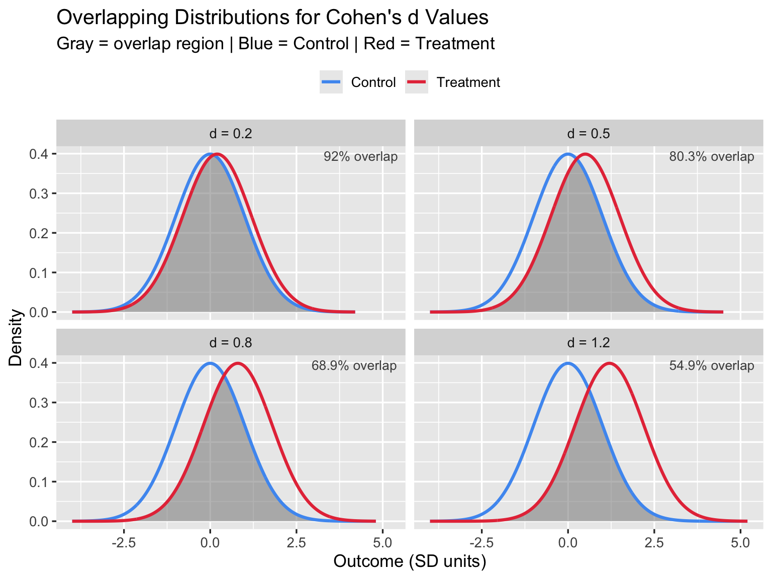
3.2 Common Language Effect Size
The Common Language Effect Size (CLES), also called Probability of Superiority, asks: if you pick one treated and one untreated patient at random, what is the probability the treated patient scores better?
\[\text{CLES} = P(X_{\text{trt}} > X_{\text{ctrl}}) = \Phi\!\left(\frac{d}{\sqrt{2}}\right)\]
d_seq  <- seq(0, 2, by = 0.01)
cles   <- pnorm(d_seq / sqrt(2))

ggplot(data.frame(d = d_seq, cles = cles), aes(x = d, y = cles)) +
  geom_line(color = "#E63946", linewidth = 1.4) +
  geom_hline(yintercept = 0.5, linetype = "dashed", color = "gray50") +
  geom_vline(xintercept = c(0.2, 0.5, 0.8), linetype = "dotted",
             color = "#4E9AF1", linewidth = 0.8) +
  annotate("text", x = 0.20, y = 0.525, label = "small\nd=0.2",
           hjust = -0.1, size = 3.5, color = "gray30") +
  annotate("text", x = 0.50, y = 0.590, label = "medium\nd=0.5",
           hjust = -0.1, size = 3.5, color = "gray30") +
  annotate("text", x = 0.80, y = 0.660, label = "large\nd=0.8",
           hjust = -0.1, size = 3.5, color = "gray30") +
  scale_y_continuous(labels = scales::percent, limits = c(0.45, 1)) +
  labs(title    = "Common Language Effect Size (CLES)",
       subtitle = "P(randomly chosen treated patient outperforms randomly chosen control)",
       x = "Cohen's d", y = "Probability of Superiority") +
  theme_gray(base_size = 13)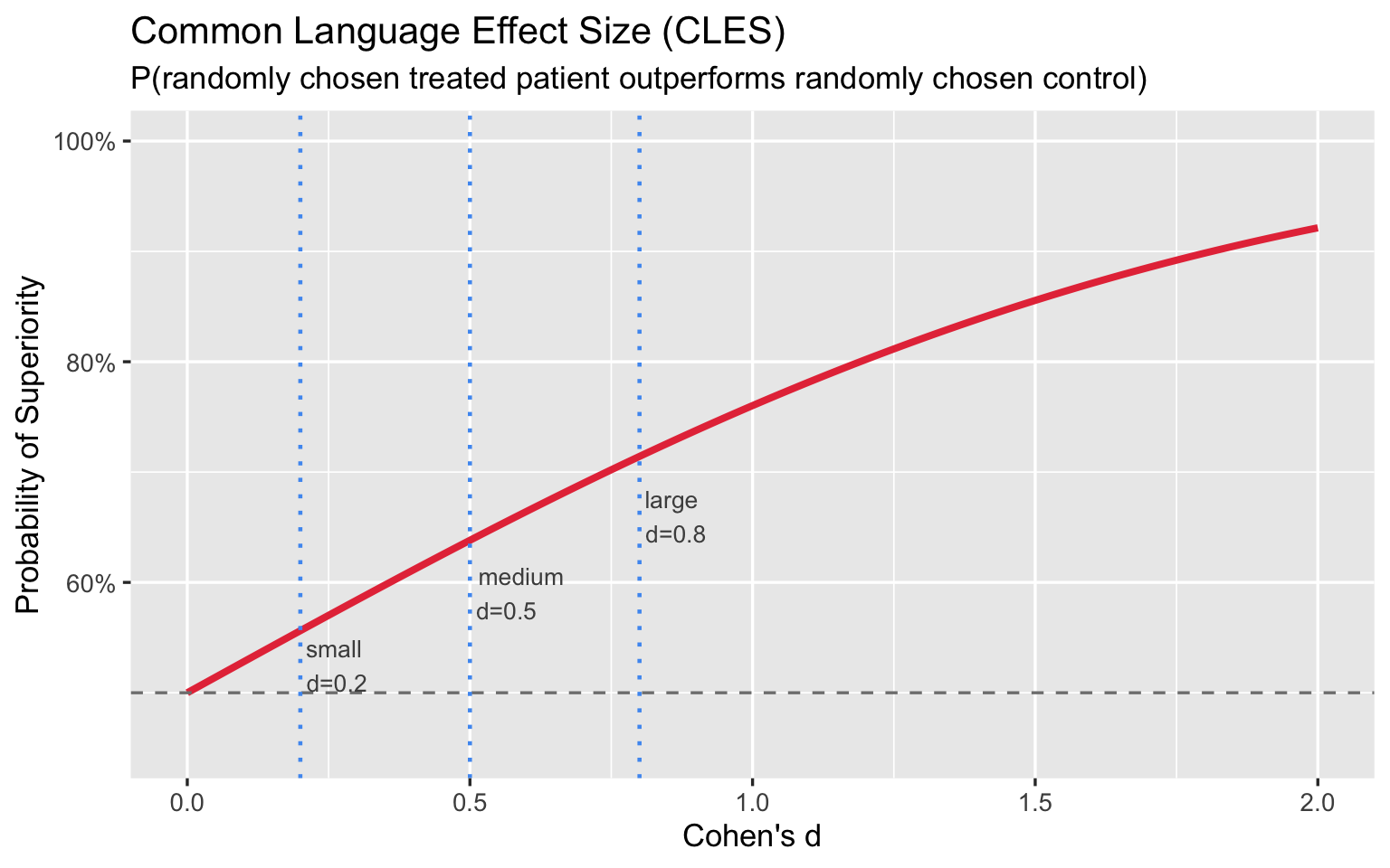
Even a “large” d = 0.8 yields only a 71% chance that a treated patient outperforms a control. Framed this way, the labels feel far less impressive.
4. Why Context Beats Benchmarks in Biomedical Research
4.1 Blood Pressure: “Medium” d, Enormous Population Impact
A first-line antihypertensive drug reduces systolic blood pressure (SBP) by 10 mmHg in a population with SD ≈ 15 mmHg — exactly the magnitude studied by Ettehad et al.
\[d = \frac{10}{15} \approx 0.67 \quad \text{("medium" by Cohen)}\]
Per the landmark Ettehad et al. (2016) Lancet meta-analysis — 123 RCTs, 613,815 participants — this 10 mmHg SBP reduction is associated with:
- −27% relative risk of stroke (RR 0.73, 95% CI 0.68–0.77)
- −17% relative risk of ischaemic heart disease (RR 0.83, 95% CI 0.78–0.88)
- −13% all-cause mortality (RR 0.87, 95% CI 0.84–0.91)
Ettehad D, Emdin CA, Kiran A, et al. Blood pressure lowering for prevention of cardiovascular disease and death: a systematic review and meta-analysis. Lancet. 2016;387(10022):957–967. doi:10.1016/S0140-6736(15)01225-8
Cohen defined a “medium” effect as one “visible to the naked eye” — his example was the IQ difference between clerks and managers. By his own framing, d = 0.67 is noticeable but unremarkable. Yet this unremarkable effect prevents more than a quarter of all strokes at the population level. The label “medium” carries no clinical information. As with “small,” the absolute benefit depends on baseline risk and the size of the exposed population — not on where d falls relative to a 1960s behavioural-science benchmark.
set.seed(123)
n_bp <- 600
ctrl_sbp <- rnorm(n_bp, 140, 15)
trt_sbp  <- rnorm(n_bp, 130, 15)
d_bp     <- cohens_d(ctrl_sbp, trt_sbp)

bp_df <- data.frame(
  SBP   = c(ctrl_sbp, trt_sbp),
  Group = rep(c("Control (μ = 140 mmHg)", "Drug (μ = 130 mmHg)"), each = n_bp)
)

ggplot(bp_df, aes(x = SBP, fill = Group)) +
  geom_histogram(alpha = 0.65, binwidth = 3, position = "identity") +
  geom_vline(xintercept = c(mean(ctrl_sbp), mean(trt_sbp)),
             color = c("#4E9AF1", "#E63946"), linewidth = 1.2, linetype = "dashed") +
  scale_fill_manual(values = c("#4E9AF1", "#E63946")) +
  labs(
    title    = sprintf('10 mmHg SBP Reduction: d = %.2f — "Medium" by Cohen, −27%% Stroke Risk at Scale', d_bp),
    subtitle = "N = 600 per group | Groups overlap heavily; population impact is determined by baseline risk, not d",
    x = "Systolic Blood Pressure (mmHg)", y = "Count", fill = NULL
  ) +
  theme_gray(base_size = 13) +
  theme(legend.position = "top")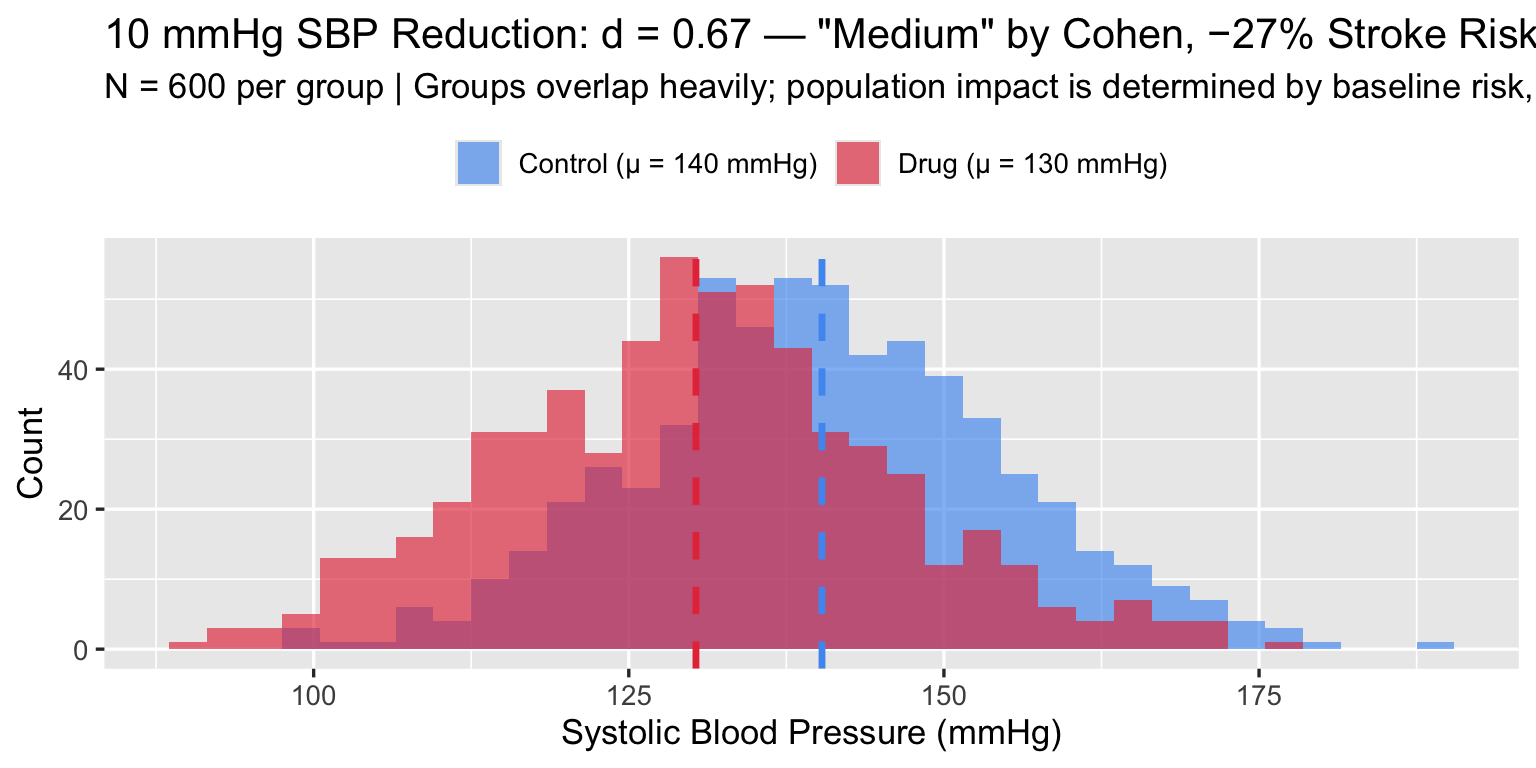
4.2 Antidepressants: The Ongoing Debate
Kirsch et al. (2008) analysed 35 trials submitted to the FDA (3,292 patients on active drug, 1,841 on placebo) and found a mean drug–placebo difference of 1.80 HDRS points (Cohen’s d = 0.32). Cipriani et al. (2018), a network meta-analysis of 522 RCTs and 116,477 patients across 21 antidepressants, found all drugs outperformed placebo; ORs for treatment response ranged from 1.37 (reboxetine) to 2.13 (amitriptyline), with a pooled SMD across drugs of approximately 0.30. Together these place the class effect at d ≈ 0.3 on the HDRS-17 (range 0–52).
Kirsch I, Deacon BJ, Huedo-Medina TB, Scoboria A, Moore TJ, Johnson BT. Initial severity and antidepressant benefits: a meta-analysis of data submitted to the Food and Drug Administration. PLoS Med. 2008;5(2):e45. doi:10.1371/journal.pmed.0050045
Cipriani A, Furukawa TA, Salanti G, et al. Comparative efficacy and acceptability of 21 antidepressant drugs for the acute treatment of adults with major depressive disorder: a systematic review and network meta-analysis. Lancet. 2018;391(10128):1357–1366. doi:10.1016/S0140-6736(17)32802-7
The MCID for HDRS-17 is debated; NICE and the FDA have used 3 points as a lower bound for clinical significance (literature range: 3–5 points). A d = 0.3 corresponds to roughly a 2.4-point difference at the pooled SD of ≈ 8 — just below this threshold, which is the crux of the ongoing debate.
set.seed(99)
n_ad    <- 400
placebo <- rnorm(n_ad, mean = 12, sd = 8)   # residual symptoms after 8 weeks
drug    <- rnorm(n_ad, mean = 9.6, sd = 8)  # d ≈ 0.3

d_ad <- cohens_d(placebo, drug)

ad_df <- data.frame(
  HDRS  = c(placebo, drug),
  Group = rep(c("Placebo", "Antidepressant"), each = n_ad)
)

ggplot(ad_df, aes(x = HDRS, fill = Group)) +
  geom_histogram(alpha = 0.65, binwidth = 2, position = "identity") +
  geom_vline(xintercept = c(mean(placebo), mean(drug)),
             color = c("#4E9AF1", "#E63946"), linewidth = 1.2, linetype = "dashed") +
  scale_fill_manual(values = c("#4E9AF1", "#E63946")) +
  labs(
    title    = sprintf("Antidepressant vs Placebo: d = %.2f on HDRS-17", d_ad),
    subtitle = "Mean difference ≈ 2.4 points | MCID threshold ≈ 3 points | Interpretation requires clinical context",
    x = "Hamilton Depression Rating Scale (HDRS-17)", y = "Count", fill = NULL
  ) +
  theme_gray(base_size = 13) +
  theme(legend.position = "top")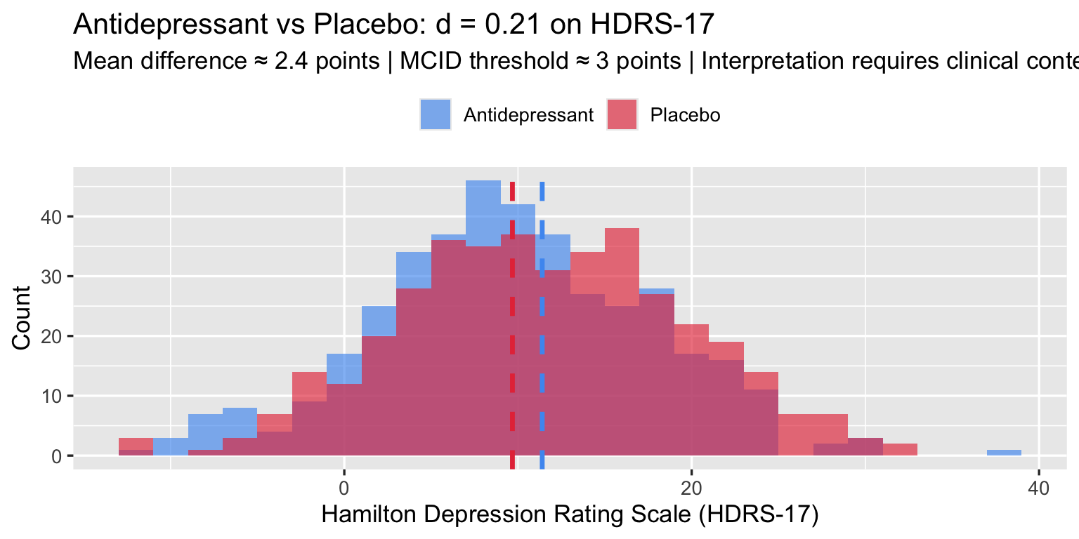
The clinical debate hinges not on d but on whether a 2.4-point HDRS difference is detectable to patients — the MCID question. Cohen’s label (“small”) adds no information to that debate.
4.3 The Sample-Size Trap
The p-value of a t-test is a function of both d and N. With enough patients, any d — no matter how small — becomes “statistically significant.” The converse is also true: a meaningful effect can remain non-significant in an underpowered study.
set.seed(7)
d_fixed  <- 0.3      # clinically debatable but plausible
n_vals   <- c(20, 30, 50, 75, 100, 150, 200, 350, 500, 1000, 2000, 5000)
alpha    <- 0.05

# Simulate one dataset per N, extract p-value
p_vals <- sapply(n_vals, function(n) {
  t.test(rnorm(n, d_fixed, 1), rnorm(n, 0, 1))$p.value
})

trap_df <- data.frame(n = n_vals, p = p_vals,
                      sig = ifelse(p_vals < alpha, "p < 0.05", "p ≥ 0.05"))

ggplot(trap_df, aes(x = n, y = p, color = sig)) +
  geom_hline(yintercept = alpha, linetype = "dashed", color = "gray40") +
  geom_line(color = "gray60", linewidth = 0.8) +
  geom_point(size = 3.5) +
  scale_x_log10(breaks = n_vals, labels = scales::comma) +
  scale_y_log10(labels = scales::number_format(accuracy = 0.001)) +
  scale_color_manual(values = c("p < 0.05" = "#E63946", "p ≥ 0.05" = "#4E9AF1")) +
  annotate("text", x = 5000, y = 0.065, label = "α = 0.05",
           hjust = 1, color = "gray30", size = 3.5) +
  labs(title    = sprintf("The Sample-Size Trap: True d = %.1f — Eventually Everything is 'Significant'", d_fixed),
       subtitle = "One simulated experiment per N | p-value (log scale) | Both axes log-transformed",
       x = "Sample size per arm (log scale)", y = "p-value (log scale)", color = NULL) +
  theme_gray(base_size = 13) +
  theme(legend.position = "top")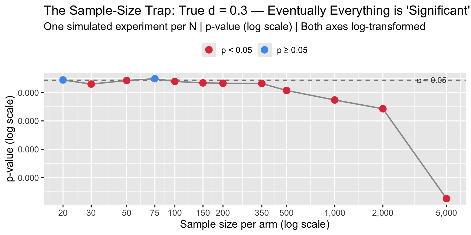
A journal that screens for p < 0.05 is really screening for d × √N > threshold. Large trials will always pass. Underpowered trials that pass are likely reporting inflated d due to winner’s curse.
5. Variants and Corrections
5.1 Hedges’ g — Small Samples
Cohen’s d is biased upward in small samples (overestimates the true effect). Hedges’ g applies a bias correction:
\[g = d \times J(df), \quad J(df) = 1 - \frac{3}{4 \cdot df - 1}\]
where \(df = n_1 + n_2 - 2\).
hedges_g <- function(x1, x2) {
  d  <- cohens_d(x1, x2)
  df <- length(x1) + length(x2) - 2
  J  <- 1 - 3 / (4 * df - 1)
  d * J
}

# Bias matters most in small samples
set.seed(55)
for (n in c(5, 10, 20, 50, 200)) {
  x1 <- rnorm(n, 0.5, 1)
  x2 <- rnorm(n, 0,   1)
  d  <- cohens_d(x1, x2)
  g  <- hedges_g(x1, x2)
  cat(sprintf("n = %4d  |  d = %+.3f  |  g = %+.3f  |  bias = %.3f\n",
              n, d, g, d - g))
}
## n = 5 | d = -0.324 | g = -0.292 | bias = -0.031
## n = 10 | d = +0.209 | g = +0.200 | bias = 0.009
## n = 20 | d = +0.806 | g = +0.790 | bias = 0.016
## n = 50 | d = +0.624 | g = +0.619 | bias = 0.005
## n = 200 | d = +0.575 | g = +0.574 | bias = 0.001Use Hedges’ g whenever \(n < 50\) per group. For typical Phase III RCTs (\(n \geq 100\)), the correction is negligible.
5.2 Glass’s Δ — Unequal Group SDs
When the two groups have meaningfully different SDs — common when one group is a patient sample and the other is a healthy control — Glass’s Δ uses only the control group SD as the denominator:
\[\Delta = \frac{\mu_1 - \mu_2}{\sigma_{\text{control}}}\]
This preserves the interpretive reference: “how many control-group SDs apart are the means?”
glass_delta <- function(x_trt, x_ctrl) {
  (mean(x_trt) - mean(x_ctrl)) / sd(x_ctrl)
}

# Hypothetical: disease group has higher variance (common in medicine)
set.seed(88)
healthy  <- rnorm(200, mean = 100, sd = 10)  # tight control group
patients <- rnorm(200, mean = 115, sd = 25)  # inflated variance with disease

cat("Cohen's d: ", round(cohens_d(patients, healthy), 3), "\n")
## Cohen's d: 0.873cat("Glass's Δ: ", round(glass_delta(patients, healthy), 3), "\n")## Glass's Δ: 1.595cat("(Using control SD = ", round(sd(healthy), 1), " vs pooled SD = ",
round(sqrt((var(healthy) + var(patients))/2), 1), ")\n")## (Using control SD = 10 vs pooled SD = 18.2 )5.3 Confidence Intervals for d
A single d without a CI is insufficient for any biomedical paper. The standard approximate CI uses:
\[\text{CI} = d \pm z_{1-\alpha/2} \times \text{SE}(d)\]
set.seed(21)
studies <- data.frame(
  Study   = paste0("Study ", 1:8),
  n_each  = c(15, 25, 50, 100, 200, 50, 80, 300),
  d_true  = rep(0.4, 8)
)

results <- studies |>
  rowwise() |>
  mutate(
    x1  = list(rnorm(n_each, d_true, 1)),
    x2  = list(rnorm(n_each, 0, 1)),
    d   = cohens_d(x1, x2),
    lo  = ci_d(d, n_each, n_each)["lower"],
    hi  = ci_d(d, n_each, n_each)["upper"]
  ) |>
  ungroup() |>
  mutate(Study = factor(Study, levels = rev(Study)))

ggplot(results, aes(x = d, y = Study)) +
  geom_vline(xintercept = 0.4, linetype = "dashed", color = "gray50") +
  geom_vline(xintercept = 0,   linetype = "solid",  color = "gray80") +
  geom_errorbarh(aes(xmin = lo, xmax = hi), height = 0.3, color = "#4E9AF1", linewidth = 0.9) +
  geom_point(aes(size = n_each), color = "#E63946") +
  scale_size_continuous(range = c(2, 7), name = "N per arm") +
  annotate("text", x = 0.42, y = 0.5, label = "True d = 0.4",
           hjust = 0, color = "gray30", size = 3.5) +
  labs(title    = "Confidence Intervals for d: Same True Effect, Very Different Uncertainty",
       subtitle = "Larger studies → narrower CIs | Small studies may cross zero or wildly overestimate",
       x = "Cohen's d", y = NULL) +
  theme_gray(base_size = 13) +
  theme(legend.position = "right")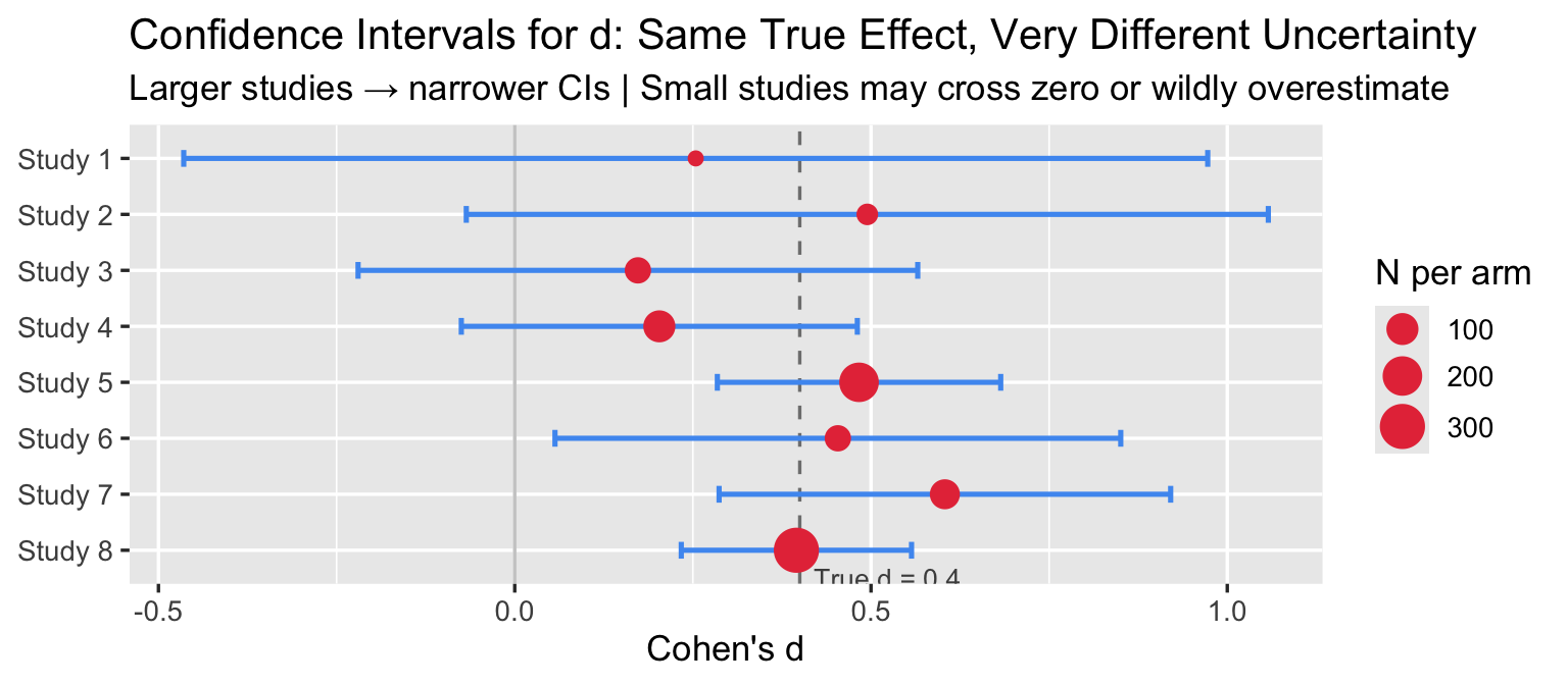
Small studies produce wide CIs that cross zero and inflated point estimates — the winner’s curse: the studies that happen to cross the significance threshold in small samples tend to overestimate d.
6. MCID: The Clinical Alternative to Cohen’s Benchmarks
The Minimal Clinically Important Difference is the smallest change in an outcome that patients (or clinicians) perceive as meaningful. Unlike Cohen’s benchmarks, MCIDs are derived empirically from patient-reported outcomes, anchor-based methods, or distribution-based methods.
mcid_df <- data.frame(
  Outcome       = c("Systolic blood pressure",
                    "HbA1c (diabetes)",
                    "HDRS-17 (depression)",
                    "SF-36 Physical Function",
                    "6-Minute Walk Distance",
                    "VAS Pain Score (0–100)",
                    "FEV₁ absolute (COPD)"),
  MCID          = c("5 mmHg", "0.5%", "3 points", "5–10 points",
                    "25–33 m", "10–15 mm", "100–140 mL"),
  `Typical SD`  = c("15 mmHg", "1.2%", "8 pts", "20 pts",
                    "90 m", "25 mm", "~300 mL"),
  `d at MCID`   = c("0.33", "0.42", "0.38", "0.25–0.50",
                    "0.31", "0.44", "0.33–0.47"),
  `Cohen label` = rep("'small'", 7)
)
knitr::kable(mcid_df, align = "llllc",
             col.names = c("Outcome", "MCID", "Typical SD",
"d at MCID", "Cohen's label"))| Outcome | MCID | Typical SD | d at MCID | Cohen’s label |
|---|---|---|---|---|
| Systolic blood pressure | 5 mmHg | 15 mmHg | 0.33 | ‘small’ |
| HbA1c (diabetes) | 0.5% | 1.2% | 0.42 | ‘small’ |
| HDRS-17 (depression) | 3 points | 8 pts | 0.38 | ‘small’ |
| SF-36 Physical Function | 5–10 points | 20 pts | 0.25–0.50 | ‘small’ |
| 6-Minute Walk Distance | 25–33 m | 90 m | 0.31 | ‘small’ |
| VAS Pain Score (0–100) | 10–15 mm | 25 mm | 0.44 | ‘small’ |
| FEV₁ absolute (COPD) | 100–140 mL | ~300 mL | 0.33–0.47 | ‘small’ |
MCID sources: SBP — Ettehad et al. 2016 Lancet; HbA1c — NICE NG28 (2015); HDRS-17 — Leucht et al. J Affect Disord* 2013;148:243–252; SF-36 PF — population-dependent, range 5–10 pts; 6MWD — Holland et al. Eur Respir J 2014;44:1428–1446; VAS Pain — Farrar et al. Pain 2001;94:149–158; FEV₁ — Donohue JF COPD 2005;2(1):111–124.*
Every MCID in the table above corresponds to a Cohen “small” effect. If a trial reports d = 0.3 for SBP but fails to mention that the MCID is 5 mmHg, the reader cannot evaluate whether the trial succeeded or failed.
Rule for biomedical reporting: report d (with 95% CI), report the MCID for the primary endpoint, and state explicitly whether the observed effect exceeds the MCID.
7. R Toolkit
7.1 Computing Effect Sizes
# All functions defined inline — no external packages needed

effect_size_summary <- function(x1, x2, label1 = "Group 1", label2 = "Group 2") {
  n1 <- length(x1);  n2 <- length(x2)
  d  <- cohens_d(x1, x2)
  g  <- hedges_g(x1, x2)
  D  <- glass_delta(x1, x2)
  cl <- pnorm(d / sqrt(2))
  ov <- 2 * pnorm(-abs(d) / 2)
  ci <- ci_d(d, n1, n2)

  cat("=== Effect Size Summary ===\n")
  cat(sprintf("  %s: n = %d, mean = %.2f, SD = %.2f\n", label1, n1, mean(x1), sd(x1)))
  cat(sprintf("  %s: n = %d, mean = %.2f, SD = %.2f\n", label2, n2, mean(x2), sd(x2)))
  cat(sprintf("  Cohen's d     = %.3f  (95%% CI: %.3f, %.3f)\n", d, ci["lower"], ci["upper"]))
  cat(sprintf("  Hedges' g     = %.3f\n", g))
  cat(sprintf("  Glass's Δ     = %.3f  (control = %s)\n", D, label2))
  cat(sprintf("  CLES          = %.1f%%  (P[%s > %s])\n", cl*100, label1, label2))
  cat(sprintf("  Overlap       = %.1f%%\n", ov*100))
}

set.seed(42)
effect_size_summary(
  rnorm(150, 130, 15),  # treatment SBP
  rnorm(150, 135, 15),  # control SBP
  label1 = "Drug", label2 = "Placebo"
)
## === Effect Size Summary ===
## Drug: n = 150, mean = 129.57, SD = 15.08
## Placebo: n = 150, mean = 134.78, SD = 14.58
## Cohen's d = -0.351 (95% CI: -0.579, -0.123)
## Hedges' g = -0.350
## Glass's Δ = -0.357 (control = Placebo)
## CLES = 40.2% (P[Drug > Placebo])
## Overlap = 86.1%7.2 Power Analysis
How many patients per arm does a trial need to detect a given d with 80% power?
power_t2 <- function(d, n, alpha = 0.05) {
  ncp    <- d * sqrt(n / 2)
  df     <- 2 * n - 2
  t_crit <- qt(1 - alpha / 2, df)
  1 - pt(t_crit, df, ncp) + pt(-t_crit, df, ncp)
}

d_targets <- c(0.2, 0.3, 0.5, 0.8)
n_range   <- seq(10, 800, by = 5)

pwr_df <- lapply(d_targets, function(d) {
  data.frame(
    d     = factor(paste0("d = ", d)),
    n     = n_range,
    power = sapply(n_range, function(n) power_t2(d, n))
  )
}) |> bind_rows()

# N needed for 80% power
n80 <- lapply(d_targets, function(d) {
  pows <- sapply(n_range, function(n) power_t2(d, n))
  n_range[which(pows >= 0.80)[1]]
})

ggplot(pwr_df, aes(x = n, y = power, color = d)) +
  geom_line(linewidth = 1.3) +
  geom_hline(yintercept = 0.80, linetype = "dashed", color = "gray40") +
  scale_y_continuous(labels = scales::percent, limits = c(0, 1)) +
  scale_color_manual(values = c("#1B5FA1", "#4E9AF1", "#E07B2A", "#E63946")) +
  annotate("text", x = 790, y = 0.825, label = "80% power target",
           hjust = 1, color = "gray30", size = 3.5) +
  labs(title    = "Power Curves for a Two-Sample t-Test (α = 0.05)",
       subtitle = sprintf("N for 80%% power: d=0.2 → %d | d=0.3 → %d | d=0.5 → %d | d=0.8 → %d",
                          n80[[1]], n80[[2]], n80[[3]], n80[[4]]),
       x = "Sample size per arm", y = "Power", color = "Effect size") +
  theme_gray(base_size = 13)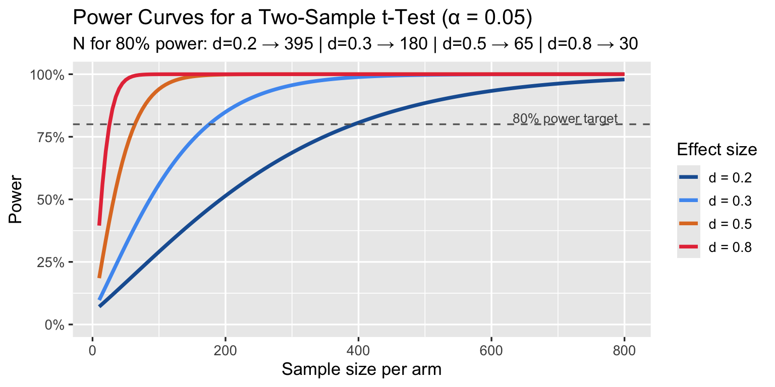
A trial powered for d = 0.5 but that actually detects d = 0.3 is underpowered by a factor of ~3. Pre-registration with explicit MCID-based power calculations is the correct approach.
8. Summary
| Topic | Key points |
|---|---|
| Cohen’s d | Standardised mean difference; dimensionless; widely reported in RCTs and meta-analyses |
| Cohen’s labels | “Small/medium/large” are arbitrary, calibrated against 1950s–60s social science, not medicine |
| Same d ≠ same importance | d = 0.33 for SBP saves lives; d = 0.33 for HDRS is debated; context is everything |
| CLES | P(treated > control) = Φ(d/√2); more intuitive than d for clinical communication |
| Sample-size trap | With N large enough, any d becomes significant; overpowered trials detect trivially small effects |
| Winner’s curse | Underpowered trials that reach p < 0.05 tend to overestimate d |
| Hedges’ g | Preferred over d when n < 50 per group; bias-corrected |
| Glass’s Δ | Preferred when group SDs differ substantially |
| CI for d | Always report; a single d without a CI is incomplete |
| MCID | The correct biomedical benchmark; derived from patient experience, not from statistical convention |
For biomedical reporting, always state: 1. Cohen’s d (or Hedges’ g) with 95% CI 2. The MCID for the primary endpoint 3. Whether the observed effect meets or exceeds the MCID