
Disease Survival Burden Assessment
# ── Change these values to re-run for any patient or disease ─────────────────

pt_age      <- 50          # Patient age at diagnosis (integer, ≥ 50)
pt_sex      <- "M"         # "M" = Male, "F" = Female
dis_name    <- "Disease X" # Short label used in plots and tables
dis_median  <- 3           # Reported median overall survival (years)
dis_ci_low  <- 1           # Lower 95% CI bound on median (years)
dis_ci_high <- 10          # Upper 95% CI bound on median (years)
Contents
- US SSA Period Life Table
- Background Population Survival
- Disease Survival Model
- Kaplan–Meier Survival Curves
- Survival Table
- Disease Burden Assessment
1. US SSA Period Life Table
The US Social Security Administration publishes annual Period Life
Tables giving the conditional probability of dying within one year \(q(x)\) and remaining life expectancy \(e(x)\) at each exact age \(x\), separately for males and females. We
use the survexp.us ratetable bundled with the
survival package, which contains the SSA Period Life Table
reformatted for survival analysis. Ages 50–99 are shown.
# survexp.us: SSA period life table as daily hazard rates (per survival package)
# Dimensions: age (one entry per year, stored in days), sex, calendar year
yr_use <- as.character(max(as.integer(dimnames(survexp.us)[[3]])))
n_ages <- dim(survexp.us)[1]

lt_all <- data.frame(
  age = seq_len(n_ages) - 1L,
  q_m = 1 - exp(-as.numeric(survexp.us[, "male",   yr_use]) * 365.25),
  q_f = 1 - exp(-as.numeric(survexp.us[, "female", yr_use]) * 365.25)
) |>
  mutate(
    l_m = round(100000 * c(1, cumprod(1 - head(q_m, -1)))),
    l_f = round(100000 * c(1, cumprod(1 - head(q_f, -1))))
  )

# Complete life expectancy ê(x) = Σ k_p_x + 0.5 (summed over remaining ages)
lt_ex_fn <- function(q) {
  n <- length(q)
  vapply(seq_len(n), function(i) round(sum(cumprod(1 - q[i:n])) + 0.5, 1), numeric(1L))
}

lt <- lt_all |>
  mutate(e_m = lt_ex_fn(q_m), e_f = lt_ex_fn(q_f)) |>
  filter(age >= 50, age <= 99) |>
  select(age, q_m, l_m, e_m, q_f, l_f, e_f)
kable(
lt |>
select(age, q_m, e_m, q_f, e_f) |>
rename(
Age = age,
`Male q(x)` = q_m,
`Male e(x)` = e_m,
`Female q(x)` = q_f,
`Female e(x)` = e_f
),
digits = 4,
caption = paste0("US SSA Period Life Table (", yr_use, ") — Ages 50–99")
)| Age | Male q(x) | Male e(x) | Female q(x) | Female e(x) |
|---|---|---|---|---|
| 50 | 0.0060 | 28.4 | 0.0035 | 32.4 |
| 51 | 0.0065 | 27.6 | 0.0038 | 31.5 |
| 52 | 0.0070 | 26.8 | 0.0041 | 30.6 |
| 53 | 0.0077 | 25.9 | 0.0045 | 29.7 |
| 54 | 0.0084 | 25.1 | 0.0049 | 28.8 |
| 55 | 0.0091 | 24.3 | 0.0053 | 28.0 |
| 56 | 0.0099 | 23.6 | 0.0057 | 27.1 |
| 57 | 0.0107 | 22.8 | 0.0062 | 26.3 |
| 58 | 0.0116 | 22.0 | 0.0067 | 25.4 |
| 59 | 0.0125 | 21.3 | 0.0073 | 24.6 |
| 60 | 0.0136 | 20.5 | 0.0079 | 23.8 |
| 61 | 0.0147 | 19.8 | 0.0086 | 23.0 |
| 62 | 0.0157 | 19.1 | 0.0092 | 22.2 |
| 63 | 0.0168 | 18.4 | 0.0098 | 21.4 |
| 64 | 0.0178 | 17.7 | 0.0105 | 20.6 |
| 65 | 0.0189 | 17.0 | 0.0111 | 19.8 |
| 66 | 0.0202 | 16.3 | 0.0119 | 19.0 |
| 67 | 0.0216 | 15.7 | 0.0129 | 18.2 |
| 68 | 0.0231 | 15.0 | 0.0140 | 17.5 |
| 69 | 0.0247 | 14.4 | 0.0153 | 16.7 |
| 70 | 0.0263 | 13.7 | 0.0167 | 15.9 |
| 71 | 0.0281 | 13.1 | 0.0183 | 15.2 |
| 72 | 0.0303 | 12.4 | 0.0200 | 14.5 |
| 73 | 0.0325 | 11.8 | 0.0217 | 13.8 |
| 74 | 0.0365 | 11.2 | 0.0245 | 13.1 |
| 75 | 0.0395 | 10.6 | 0.0269 | 12.4 |
| 76 | 0.0439 | 10.0 | 0.0299 | 11.7 |
| 77 | 0.0480 | 9.4 | 0.0330 | 11.1 |
| 78 | 0.0534 | 8.9 | 0.0371 | 10.4 |
| 79 | 0.0582 | 8.4 | 0.0412 | 9.8 |
| 80 | 0.0640 | 7.8 | 0.0459 | 9.2 |
| 81 | 0.0703 | 7.3 | 0.0511 | 8.6 |
| 82 | 0.0773 | 6.9 | 0.0571 | 8.0 |
| 83 | 0.0866 | 6.4 | 0.0642 | 7.5 |
| 84 | 0.0960 | 5.9 | 0.0724 | 7.0 |
| 85 | 0.1071 | 5.5 | 0.0815 | 6.5 |
| 86 | 0.1167 | 5.1 | 0.0900 | 6.0 |
| 87 | 0.1309 | 4.7 | 0.1019 | 5.6 |
| 88 | 0.1464 | 4.4 | 0.1150 | 5.1 |
| 89 | 0.1632 | 4.0 | 0.1294 | 4.7 |
| 90 | 0.1812 | 3.7 | 0.1452 | 4.4 |
| 91 | 0.2005 | 3.5 | 0.1623 | 4.0 |
| 92 | 0.2208 | 3.2 | 0.1807 | 3.7 |
| 93 | 0.2421 | 3.0 | 0.2004 | 3.4 |
| 94 | 0.2643 | 2.7 | 0.2212 | 3.2 |
| 95 | 0.2872 | 2.5 | 0.2431 | 2.9 |
| 96 | 0.3105 | 2.4 | 0.2658 | 2.7 |
| 97 | 0.3340 | 2.2 | 0.2892 | 2.5 |
| 98 | 0.3575 | 2.1 | 0.3131 | 2.3 |
| 99 | 0.3807 | 1.9 | 0.3372 | 2.1 |
2. Background Population Survival
From the life table we build the survival function \(S_{bg}(t)\) for a person of the specified age and sex. Starting from age \(a\), the probability of surviving at least \(t\) more years is:
\[S_{bg}(t) = \prod_{x=a}^{a+t-1}\bigl(1 - q(x)\bigr), \quad t = 0, 1, 2, \ldots\]
q_col <- if (pt_sex == "M") "q_m" else "q_f"
lt_pt <- lt |> filter(age >= pt_age)
q_x   <- lt_pt[[q_col]]

# Survival at each integer year from diagnosis
S_bg <- c(1, cumprod(1 - q_x))
t_bg <- 0L:(length(S_bg) - 1L)

# Median remaining years (first time S drops below 0.5)
bg_median <- t_bg[which(S_bg < 0.5)[1L]] - 1L

# Restricted mean survival time (RMST) over 30-year horizon
horizon <- min(30L, max(t_bg))
bg_rmst <- sum(S_bg[t_bg < horizon])   # ∫₀ᴴ S(t) dt for unit-step function
For a male aged 50, the SSA life table implies:
- Median remaining survival: 30 years (expected death near age 80)
- 30-year restricted mean survival (RMST): 24.7 years
3. Disease Survival Model
Given only a reported median and 95% CI, we fit a log-normal survival distribution, \(\log T \sim \mathcal{N}(\mu,\,\sigma^2)\).
The log-normal reproduces the stated median exactly. Its two parameters are derived as:
\[\mu = \ln(\text{median}), \qquad \sigma = \frac{\ln(\text{CI}_\text{high}) - \ln(\text{CI}_\text{low})}{2 \times 1.96}\]
The spread \(\sigma\) encodes how wide the survival distribution is — a large \(\sigma\) means high patient-to-patient variability in outcome.
mu_d    <- log(dis_median)
sigma_d <- (log(dis_ci_high) - log(dis_ci_low)) / (2 * 1.96)

# Theoretical mean of this log-normal
dis_mean_raw <- exp(mu_d + sigma_d^2 / 2)

# Disease RMST over the same horizon (fine-grid numerical integration)
t_fine     <- seq(0, horizon, by = 0.01)
S_dis_fine <- 1 - plnorm(t_fine, meanlog = mu_d, sdlog = sigma_d)
dis_rmst <- sum(diff(t_fine) * S_dis_fine[-length(S_dis_fine)])| Parameter | Value |
|---|---|
| \(\mu\) (location) | 1.099 |
| \(\sigma\) (shape) | 0.587 |
| Median (exact) | 3 years |
| Theoretical mean | 3.6 years |
| 30-year RMST | 3.6 years |
Note. \(\sigma\) is derived from the CI on the median estimate, not from patient-level heterogeneity data. It serves as a scale parameter for the shape of the modelled survival curve.
4. Kaplan–Meier Survival Curves
We generate \(n = 10{,}000\) synthetic survival times from each model and apply the standard Kaplan–Meier estimator.
- Background cohort: sampled via the inverse CDF of the SSA life table step function.
- Disease cohort: sampled from the fitted log-normal distribution; times are capped at the life-table horizon.
set.seed(2024)
n_sim <- 10000L

# Background: inverse-CDF of the step survival function
bg_times <- sapply(runif(n_sim), function(u) {
  idx <- which(S_bg <= u)
  if (length(idx) == 0L) max(t_bg) else t_bg[idx[1L]]
})

# Disease: log-normal sample, capped at life-table horizon
dis_times <- pmin(
  rlnorm(n_sim, meanlog = mu_d, sdlog = sigma_d),
  max(t_bg)
)

km_bg  <- survfit(Surv(bg_times,  rep(1L, n_sim)) ~ 1)
km_dis <- survfit(Surv(dis_times, rep(1L, n_sim)) ~ 1)
tidy_km <- function(km, label) {
data.frame(
time = c(0, km$time),
surv = c(1, km$surv),
lower = c(1, km$lower),
upper = c(1, km$upper),
group = label
)
}
bg_label <- paste0(
"Background (", ifelse(pt_sex == "M", "male", "female"), ", age ", pt_age, ")"
)
bg_df <- tidy_km(km_bg, bg_label)
# Disease CI: parametric bounds from reported median 95% CI.
# With n = 10,000 from a continuous distribution the KM CI is negligible;
# the meaningful uncertainty is in the reported median itself.
t_dis <- c(0, km_dis$time)
dis_df <- data.frame(
time = t_dis,
surv = c(1, km_dis$surv),
lower = 1 - plnorm(t_dis, log(dis_ci_high), sigma_d),
upper = 1 - plnorm(t_dis, log(dis_ci_low), sigma_d),
group = dis_name
)
plot_df <- rbind(bg_df, dis_df)
curve_colors <- setNames(c("#2470b3", "#902000"), c(bg_label, dis_name))
curve_types <- setNames(c("solid", "dashed"), c(bg_label, dis_name))
ggplot(plot_df, aes(x = time, y = surv * 100, color = group, linetype = group)) +
geom_ribbon(aes(ymin = lower * 100, ymax = upper * 100, fill = group),
alpha = 0.15, color = NA) +
geom_step(linewidth = 0.85) +
scale_color_manual(values = curve_colors) +
scale_fill_manual(values = curve_colors) +
scale_linetype_manual(values = curve_types) +
geom_hline(yintercept = 50, color = "gray55", linetype = "dotted", linewidth = 0.4) +
annotate("text", x = horizon * 0.97, y = 53, label = "50%",
hjust = 1, size = 3.2, color = "gray50") +
scale_x_continuous(limits = c(0, horizon), breaks = seq(0, horizon, by = 5)) +
scale_y_continuous(limits = c(0, 101), breaks = seq(0, 100, by = 20)) +
labs(
title = paste0(dis_name, " — Survival vs Background Population"),
subtitle = paste0(
ifelse(pt_sex == "M", "Male", "Female"), ", age at diagnosis ", pt_age,
" | Disease median ", dis_median,
" yr (95% CI ", dis_ci_low, "–", dis_ci_high, " yr)"
),
x = "Years from diagnosis",
y = "Survival (%)",
color = NULL, linetype = NULL,
caption = paste0(
"Background 95% CI: Greenwood formula (KM, n = ", format(n_sim, big.mark = ","), "). ",
"Disease 95% CI: log-normal survival at reported median CI bounds (",
dis_ci_low, "–", dis_ci_high, " yr)."
)
) +
theme_gray() +
theme(legend.position = "bottom") +
guides(fill = "none")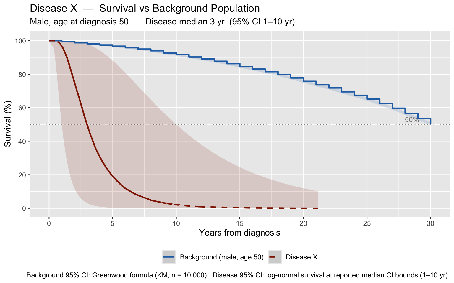
5. Survival Table
KM estimates at clinically relevant time points. The 95% CI uses Greenwood’s formula (log-log transformation).
t_pts <- c(1, 2, 3, 5, 10, 15, 20)
t_pts <- t_pts[t_pts <= horizon]

extract_km <- function(km, times) {
  s <- summary(km, times = times, extend = TRUE)
  data.frame(
    n_risk = s$n.risk,
    surv   = round(s$surv  * 100, 1),
    lower  = round(s$lower * 100, 1),
    upper  = round(s$upper * 100, 1)
  )
}

bg_tbl  <- extract_km(km_bg,  t_pts)
dis_tbl <- extract_km(km_dis, t_pts)

km_out <- data.frame(
  `Year`                            = t_pts,
  `Bg n at risk`                    = bg_tbl$n_risk,
  `Background survival % (95% CI)`  = paste0(bg_tbl$surv,
                                              " (", bg_tbl$lower, "–", bg_tbl$upper, ")"),
  `Dis n at risk`                   = dis_tbl$n_risk,
  `Disease survival % (95% CI)`     = paste0(dis_tbl$surv,
                                             " (", dis_tbl$lower, "–", dis_tbl$upper, ")"),
  `Difference (pp)`                 = bg_tbl$surv - dis_tbl$surv,
  check.names = FALSE
)

kable(km_out,
      caption = paste0("Kaplan–Meier survival estimates — Background vs ", dis_name),
align = c("r", "r", "l", "r", "l", "r"))| Year | Bg n at risk | Background survival % (95% CI) | Dis n at risk | Disease survival % (95% CI) | Difference (pp) |
|---|---|---|---|---|---|
| 1 | 10000 | 99.4 (99.2–99.5) | 9672 | 96.7 (96.4–97.1) | 2.7 |
| 2 | 9937 | 98.8 (98.6–99) | 7517 | 75.2 (74.3–76) | 23.6 |
| 3 | 9877 | 98.1 (97.8–98.3) | 4963 | 49.6 (48.7–50.6) | 48.5 |
| 5 | 9742 | 96.7 (96.4–97.1) | 1909 | 19.1 (18.3–19.9) | 77.6 |
| 10 | 9269 | 91.6 (91.1–92.2) | 210 | 2.1 (1.8–2.4) | 89.5 |
| 15 | 8629 | 84.6 (83.9–85.3) | 37 | 0.4 (0.3–0.5) | 84.2 |
| 20 | 7777 | 75.7 (74.9–76.6) | 3 | 0 (0–0.1) | 75.7 |
6. Disease Burden Assessment
bg_km_tbl     <- summary(km_bg)$table
bg_med_km     <- round(bg_km_tbl[["median"]],  1)
bg_med_lower  <- round(bg_km_tbl[["0.95LCL"]], 1)
bg_med_upper  <- round(bg_km_tbl[["0.95UCL"]], 1)

dis_km_tbl    <- summary(km_dis)$table
dis_med_km    <- round(dis_km_tbl[["median"]],  1)
dis_med_lower <- round(dis_km_tbl[["0.95LCL"]], 1)
dis_med_upper <- round(dis_km_tbl[["0.95UCL"]], 1)

yll_med  <- round(bg_med_km - dis_median, 1)
yll_rmst <- round(bg_rmst   - dis_rmst,   1)

burden_tbl <- data.frame(
  Metric = c(
    paste0("Median remaining survival — background (",
           ifelse(pt_sex == "M", "male", "female"), ", age ", pt_age, ")"),
    paste0("Median overall survival — ", dis_name),
    "Years of life lost  (median comparison)",
    paste0(horizon, "-yr RMST — background"),
    paste0(horizon, "-yr RMST — ", dis_name),
    paste0("Years of life lost  (", horizon, "-yr RMST comparison)")
  ),
  Estimate = c(
    paste0(bg_med_km,  " years  (95% CI ", bg_med_lower, "–", bg_med_upper,
           " yr;  to age ≈", pt_age + as.integer(bg_med_km), ")"),
    paste0(dis_median, " years  (95% CI ", dis_ci_low, "–", dis_ci_high, " yr)"),
    paste0(yll_med,  " years"),
    paste0(round(bg_rmst,  1), " years"),
    paste0(round(dis_rmst, 1), " years"),
    paste0(yll_rmst, " years")
  ),
  stringsAsFactors = FALSE
)

kable(burden_tbl,
      col.names = c("Metric", "Estimate"),
caption = "Disease burden summary")| Metric | Estimate |
|---|---|
| Median remaining survival — background (male, age 50) | 31 years (95% CI 30–31 yr; to age ≈81) |
| Median overall survival — Disease X | 3 years (95% CI 1–10 yr) |
| Years of life lost (median comparison) | 28 years |
| 30-yr RMST — background | 24.7 years |
| 30-yr RMST — Disease X | 3.6 years |
| Years of life lost (30-yr RMST comparison) | 21.1 years |
A male aged 50 without the disease has an expected median remaining survival of 31 years (95% CI 30–31 yr; to near age 81), per the US SSA Period Life Table.
With Disease X (median OS 3 yr, 95% CI 1–10 yr), the estimated years of life lost are:
- 28 years comparing medians
- 21.1 years comparing 30-year restricted mean survival times
Interpretation. The disease survival curve represents overall survival as typically reported from clinical trials, incorporating background mortality. The background curve is the expected survival of a matched general-population individual. The gap between the two curves is the attributable disease burden. To update this analysis, change the six parameters in the first code chunk (
params) and re-knit.