
ILD Biopsy Decision Analysis
Clinical context
All patients with suspected Interstitial Lung Disease (ILD) undergo sequential biopsy:
- Cryobiopsy — first procedure for every patient
- Surgical Lung Biopsy (SLB) — performed on every patient regardless of cryobiopsy result
A Monte Carlo simulation (N = 10,000, set.seed(2024))
propagates diagnostic uncertainty through the full pathway and samples
procedural complication rates from their probability distributions.
Parameters
set.seed(2024)
N <- 10000

# Cryobiopsy
p_cryo <- c(high = 0.60, low = 0.31, nil = 0.09)

# Surgical biopsy (conditional on cryo result)

# After HIGH confidence cryo: 95% + 2.5% + 2.5% = 100%
p_surg_high <- c(
  concordant    = 0.950,
  disc_uncl     = 0.025,
  disc_hc_other = 0.025
)

# After LOW confidence cryo: 60% concordant + 20% unclassifiable + 20% HC other = 100%
p_surg_low <- c(
  concordant    = 0.60,
  disc_uncl     = 0.20,
  disc_hc_other = 0.20
)

# After NONINFORMATIVE cryo: 17% concordant + 83% discordant = 100%
# Within the 83% discordant: 60% LC other + 40% HC other
p_surg_nil <- c(
  concordant    = 0.170,
  disc_lc_other = 0.83 * 0.60,   # 49.8%
  disc_hc_other = 0.83 * 0.40    # 33.2%
)

# Complication rates
p_cryo_ptx     <- 0.08   # cryobiopsy pneumothorax
p_surg_airleak <- 0.05   # surgical persistent air leak

# Surgical mortality: Beta(4, 96) → mean 4%, 95% CI ≈ 2–8%
surg_mort_alpha <- 4
surg_mort_beta  <- 96

# Label maps (used throughout)
cryo_labels <- c(high = "High confidence", low = "Low confidence", nil = "Noninformative")
surg_labels  <- c(
  concordant    = "Concordant",
  disc_uncl     = "Discordant – Unclassifiable",
  disc_hc_other = "Discordant – HC other Dx",
  disc_lc_other = "Discordant – LC other Dx"
)
surg_colors  <- c(
  concordant    = "#1A8A4A",
  disc_uncl     = "#CA6F1E",
  disc_hc_other = "#B03A2E",
  disc_lc_other = "#D68910"
)
Decision tree (theoretical probabilities)
# Theoretical expected n per leaf (for node labels)
n_high <- round(N * p_cryo["high"])
n_low  <- round(N * p_cryo["low"])
n_nil  <- round(N * p_cryo["nil"])

fmt <- function(n, p) sprintf("%.1f%%\n(exp. n≈%d)", p * 100, round(n * p))

grViz(paste0('
digraph ILD {
  graph [layout=dot, rankdir=LR, fontname="Helvetica", nodesep=0.4, ranksep=1.0]
  node  [shape=rectangle, style="filled,rounded", fontname="Helvetica", fontsize=10, margin="0.12,0.07"]
  edge  [fontname="Helvetica", fontsize=9, color="#555555"]

  ROOT [label="ALL PATIENTS\nN = 10,000\nCryobiopsy →", fillcolor="#2471A3", fontcolor=white, shape=ellipse, fontsize=11]

  C_H [label="High confidence\n60%  (n≈60,00)", fillcolor="#1A8A4A", fontcolor=white]
  C_L [label="Low confidence\n31%  (n≈31,00)", fillcolor="#D68910", fontcolor=white]
  C_N [label="Noninformative\n9%   (n≈9,00)",  fillcolor="#B03A2E", fontcolor=white]

  SH1 [label="Concordant\n95.0%", fillcolor="#2ECC71", fontcolor=white]
  SH2 [label="Discordant\nUnclassifiable\n2.5%", fillcolor="#CA6F1E", fontcolor=white]
  SH3 [label="Discordant\nHC other Dx\n2.5%", fillcolor="#E74C3C", fontcolor=white]

  SL1 [label="Concordant\n60%", fillcolor="#2ECC71", fontcolor=white]
  SL3 [label="Discordant\nUnclassifiable\n20%", fillcolor="#CA6F1E", fontcolor=white]
  SL4 [label="Discordant\nHC other Dx\n20%", fillcolor="#E74C3C", fontcolor=white]

  SN1 [label="Concordant\n17.0%",  fillcolor="#2ECC71", fontcolor=white]
  SN2 [label="Discordant\nLC other Dx\n49.8%", fillcolor="#D68910", fontcolor=white]
  SN3 [label="Discordant\nHC other Dx\n33.2%", fillcolor="#E74C3C", fontcolor=white]

  COMP [label="Complications\n• Cryo pneumothorax 8%\n• SLB mortality 4% (95%CI 2–8%)\n• SLB air leak 5%",
        fillcolor="#6C3483", fontcolor=white, shape=note, fontsize=9]

  ROOT -> C_H [label=" 60%"]
  ROOT -> C_L [label=" 31%"]
  ROOT -> C_N [label="  9%"]

  C_H -> SH1 [label=" 95.0%"]
  C_H -> SH2 [label=" 2.5%"]
  C_H -> SH3 [label=" 2.5%"]

  C_L -> SL1 [label=" 60%"]
  C_L -> SL3 [label=" 20%"]
  C_L -> SL4 [label=" 20%"]

  C_N -> SN1 [label=" 17.0%"]
  C_N -> SN2 [label=" 49.8%"]
  C_N -> SN3 [label=" 33.2%"]

  ROOT -> COMP [style=dashed, color="#6C3483", label="  all\n  patients"]
}
'))
Monte Carlo simulation
# Step 1 — cryobiopsy result
cryo <- sample(names(p_cryo), N, replace = TRUE, prob = p_cryo)

# Step 2 — cryo complication (pneumothorax)
ptx <- rbinom(N, 1, p_cryo_ptx) == 1

# Step 3 — surgical biopsy result conditional on cryo result
surg <- character(N)
surg[cryo == "high"] <- sample(names(p_surg_high), sum(cryo == "high"), TRUE, p_surg_high)
surg[cryo == "low"]  <- sample(names(p_surg_low),  sum(cryo == "low"),  TRUE, p_surg_low)
surg[cryo == "nil"]  <- sample(names(p_surg_nil),  sum(cryo == "nil"),  TRUE, p_surg_nil)

# Step 4 — surgical complications
# Per-patient mortality probability drawn from Beta prior (propagates parameter uncertainty)
mort_p  <- rbeta(N, surg_mort_alpha, surg_mort_beta)
died    <- rbinom(N, 1, mort_p) == 1
airleak <- rbinom(N, 1, p_surg_airleak) == 1

sim <- tibble(
  patient = seq_len(N),
  cryo, ptx, surg, mort_p, died, airleak
)

cat("Simulation complete:", N, "patients\n")
## Simulation complete: 10000 patientscat("Cryo breakdown —",
sum(cryo=="high"), "high /",
sum(cryo=="low"), "low /",
sum(cryo=="nil"), "noninformative\n")## Cryo breakdown — 6025 high / 3089 low / 886 noninformativecat("Complications — pneumothorax:", sum(ptx),
"| surgical deaths:", sum(died),
"| air leak:", sum(airleak), "\n")## Complications — pneumothorax: 815 | surgical deaths: 401 | air leak: 533Results
Cryobiopsy outcome distribution
cryo_colors_vec <- c(high = "#1A8A4A", low = "#D68910", nil = "#B03A2E")

sim %>%
  count(cryo) %>%
  mutate(label = cryo_labels[cryo], pct = n / N) %>%
  ggplot(aes(x = reorder(label, -pct), y = pct, fill = cryo)) +
  geom_col(show.legend = FALSE, width = 0.55) +
  geom_text(aes(label = sprintf("n = %d\n%.1f%%", n, pct * 100)),
            vjust = -0.4, size = 4) +
  scale_fill_manual(values = cryo_colors_vec) +
  scale_y_continuous(labels = percent, limits = c(0, 0.75),
                     expand = expansion(mult = c(0, 0.12))) +
  labs(title = "Cryobiopsy results  (N = 10,000)",
       x = NULL, y = "Proportion of patients") +
  theme_minimal(base_size = 13) +
  theme(plot.title = element_text(face = "bold"))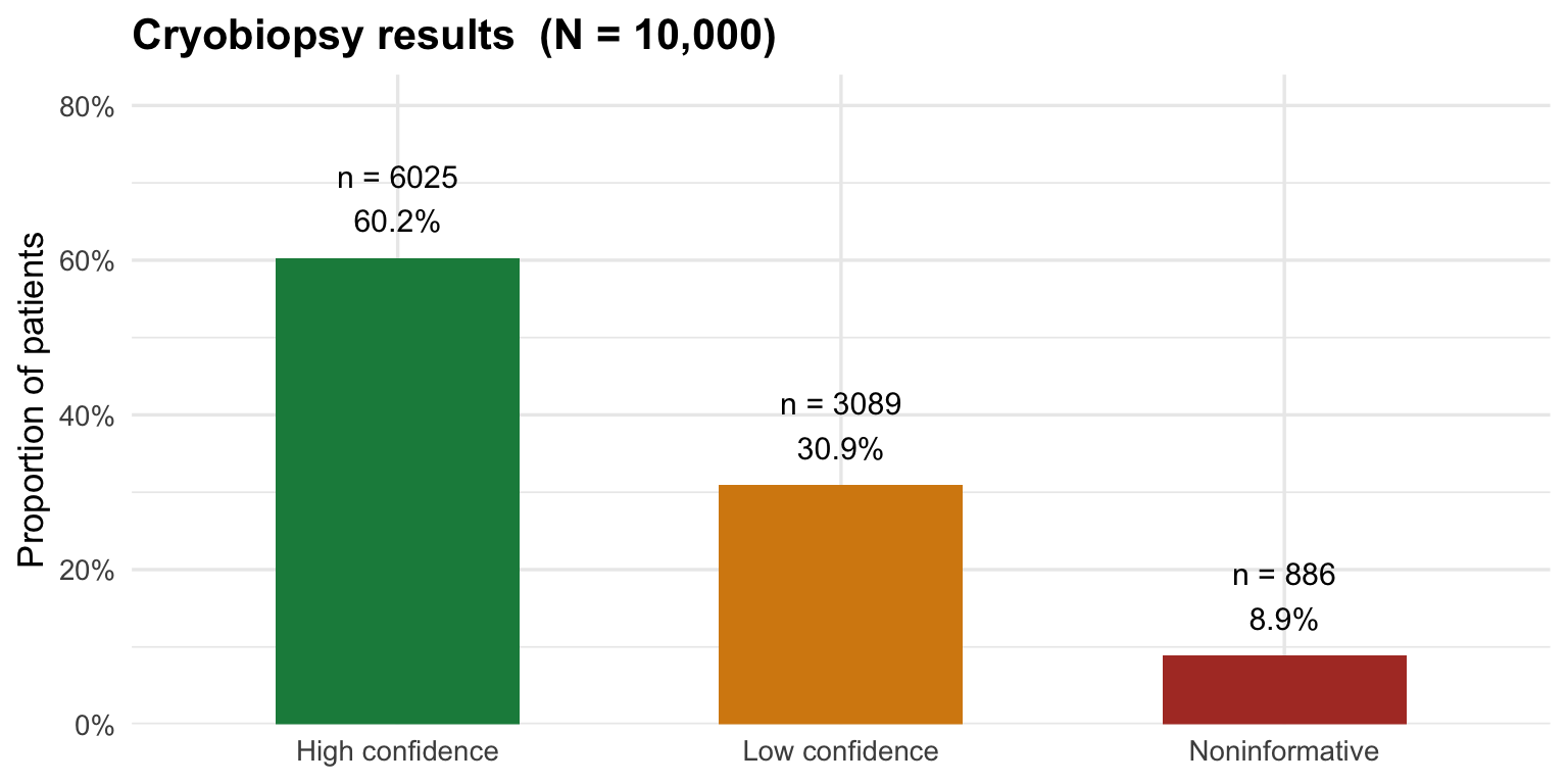
Surgical biopsy outcomes by cryo group
sim %>%
  count(cryo, surg) %>%
  group_by(cryo) %>%
  mutate(
    pct      = n / sum(n),
    surg_lbl = surg_labels[surg],
    cryo_lbl = sprintf("%s cryo\n(n = %d)", cryo_labels[cryo], sum(n))
  ) %>%
  ungroup() %>%
  ggplot(aes(x = reorder(surg_lbl, pct), y = pct, fill = surg)) +
  geom_col(show.legend = FALSE) +
  geom_text(aes(label = sprintf("%.1f%%  (n = %d)", pct * 100, n)),
            hjust = -0.08, size = 3.2) +
  coord_flip() +
  facet_wrap(~ cryo_lbl, scales = "free_y", ncol = 1) +
  scale_y_continuous(labels = percent, limits = c(0, 1.12),
                     expand = expansion(mult = c(0, 0))) +
  scale_fill_manual(values = surg_colors) +
  labs(title = "Surgical biopsy outcomes by cryobiopsy group",
       x = NULL, y = "Proportion within cryo group") +
  theme_minimal(base_size = 12) +
  theme(plot.title = element_text(face = "bold"),
        strip.text = element_text(face = "bold", size = 11),
        panel.spacing = unit(1, "lines"))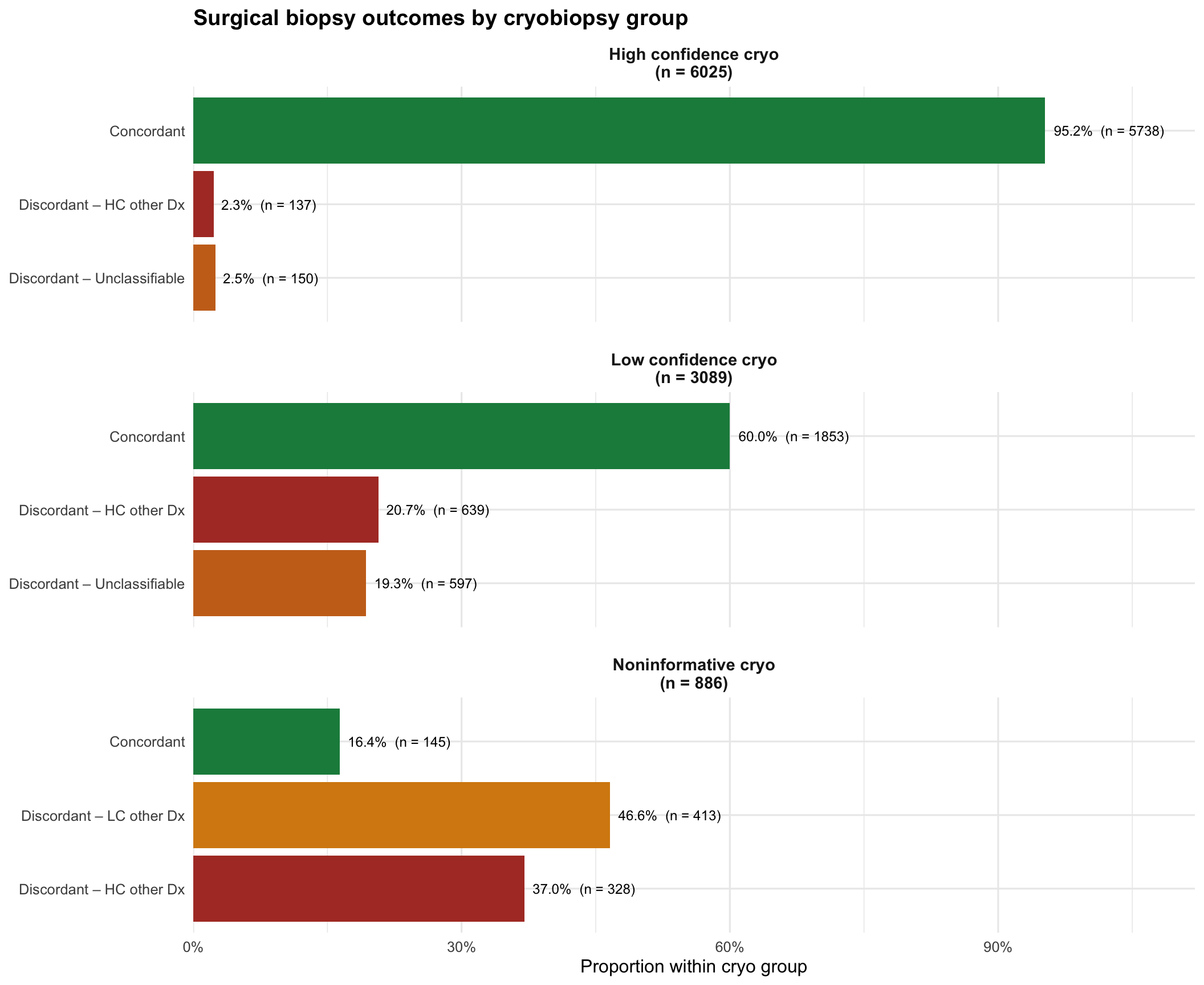
Final diagnostic outcomes — entire cohort
final_cats <- c(
  concordant    = "Concordant",
  disc_uncl     = "Discordant – Unclassifiable",
  disc_hc_other = "Discordant – HC other Dx",
  disc_lc_other = "Discordant – LC other Dx"
)
final_colors <- c(
  "Concordant"                  = "#1A8A4A",
  "Discordant – Unclassifiable" = "#CA6F1E",
  "Discordant – HC other Dx"    = "#B03A2E",
  "Discordant – LC other Dx"    = "#D68910"
)

sim %>%
  mutate(outcome = final_cats[surg]) %>%
  count(outcome) %>%
  mutate(pct = n / N) %>%
  arrange(desc(pct)) %>%
  ggplot(aes(x = reorder(outcome, pct), y = pct, fill = outcome)) +
  geom_col(show.legend = FALSE, width = 0.65) +
  geom_text(aes(label = sprintf("n = %d   (%.1f%%)", n, pct * 100)),
            hjust = -0.05, size = 3.6) +
  coord_flip() +
  scale_y_continuous(labels = percent, limits = c(0, 0.82),
                     expand = expansion(mult = c(0, 0))) +
  scale_fill_manual(values = final_colors) +
  labs(title = "Final diagnostic outcomes — all 10,000 patients",
       subtitle = "After cryobiopsy + surgical lung biopsy",
       x = NULL, y = "Proportion of total cohort") +
  theme_minimal(base_size = 12) +
  theme(plot.title = element_text(face = "bold"))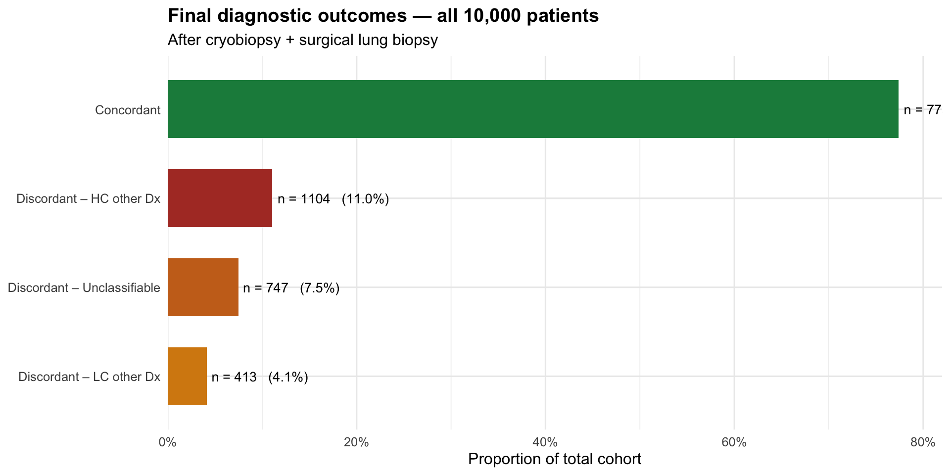
Complication analysis
comp_df <- tibble(
  label     = c("Cryo\nPneumothorax", "SLB\nMortality", "SLB\nAir leak"),
  n         = c(sum(sim$ptx), sum(sim$died), sum(sim$airleak)),
  rate_theo = c(p_cryo_ptx, surg_mort_alpha / (surg_mort_alpha + surg_mort_beta), p_surg_airleak),
  fill_col  = c("#9B59B6", "#6C3483", "#A569BD")
) %>%
  mutate(
    pct  = n / N,
    ci_l = map_dbl(n, ~ binom.test(.x, N)$conf.int[1]),
    ci_h = map_dbl(n, ~ binom.test(.x, N)$conf.int[2])
  )

p_comp <- ggplot(comp_df, aes(x = label, y = pct, fill = label)) +
  geom_col(show.legend = FALSE, width = 0.5) +
  geom_errorbar(aes(ymin = ci_l, ymax = ci_h), width = 0.12, linewidth = 0.9) +
  geom_point(aes(y = rate_theo), shape = 18, size = 4, color = "black") +
  geom_text(aes(y = ci_h, label = sprintf("n=%d\n%.1f%%", n, pct * 100)),
            vjust = -0.5, size = 3.5) +
  scale_fill_manual(values = setNames(comp_df$fill_col, comp_df$label)) +
  scale_y_continuous(labels = percent, limits = c(0, 0.14),
                     expand = expansion(mult = c(0, 0.12))) +
  labs(title = "Complication rates",
       subtitle = "Bars = simulated; ◆ = theoretical rate; error bars = 95% CI (Wilson)",
       x = NULL, y = "Rate") +
  theme_minimal(base_size = 12) +
  theme(plot.title = element_text(face = "bold"))

# Surgical mortality prior (Beta distribution)
beta_df <- tibble(
  x    = seq(0, 0.14, length.out = 600),
  dens = dbeta(x, surg_mort_alpha, surg_mort_beta)
)
ci_lo <- qbeta(0.025, surg_mort_alpha, surg_mort_beta)
ci_hi <- qbeta(0.975, surg_mort_alpha, surg_mort_beta)

p_beta <- ggplot(beta_df, aes(x = x * 100, y = dens)) +
  geom_ribbon(data = filter(beta_df, x >= ci_lo & x <= ci_hi),
              aes(ymin = 0, ymax = dens), fill = "#6C3483", alpha = 0.25) +
  geom_line(linewidth = 1.1, color = "#6C3483") +
  geom_vline(xintercept = 4, linetype = "dashed", linewidth = 0.9) +
  geom_vline(xintercept = c(ci_lo * 100, ci_hi * 100),
             linetype = "dotted", color = "grey50", linewidth = 0.8) +
  annotate("text", x = 6, y = max(beta_df$dens) * 0.85,
           label = sprintf("Mean = 4%%\n95%% CI: %.1f%%–%.1f%%", ci_lo*100, ci_hi*100),
           size = 3.5, hjust = 0) +
  labs(title = "Surgical mortality prior",
       subtitle = "Beta(4, 96) — shaded = 95% CI",
       x = "Mortality rate (%)", y = "Density") +
  theme_minimal(base_size = 12) +
  theme(plot.title = element_text(face = "bold"))

# Distribution of per-patient sampled mortality probability
p_mort_mc <- ggplot(sim, aes(x = mort_p * 100)) +
  geom_histogram(bins = 60, fill = "#6C3483", alpha = 0.7, color = "white") +
  geom_vline(xintercept = 4, linetype = "dashed", linewidth = 0.9) +
  geom_vline(xintercept = c(ci_lo * 100, ci_hi * 100),
             linetype = "dotted", color = "grey50", linewidth = 0.8) +
  labs(title = "Monte Carlo: sampled mortality probabilities",
       subtitle = sprintf("Simulated deaths: n = %d (%.1f%%)", sum(sim$died), mean(sim$died)*100),
       x = "Per-patient mortality rate (%)", y = "Patients (n)") +
  theme_minimal(base_size = 12) +
  theme(plot.title = element_text(face = "bold"))

p_comp | p_beta | p_mort_mc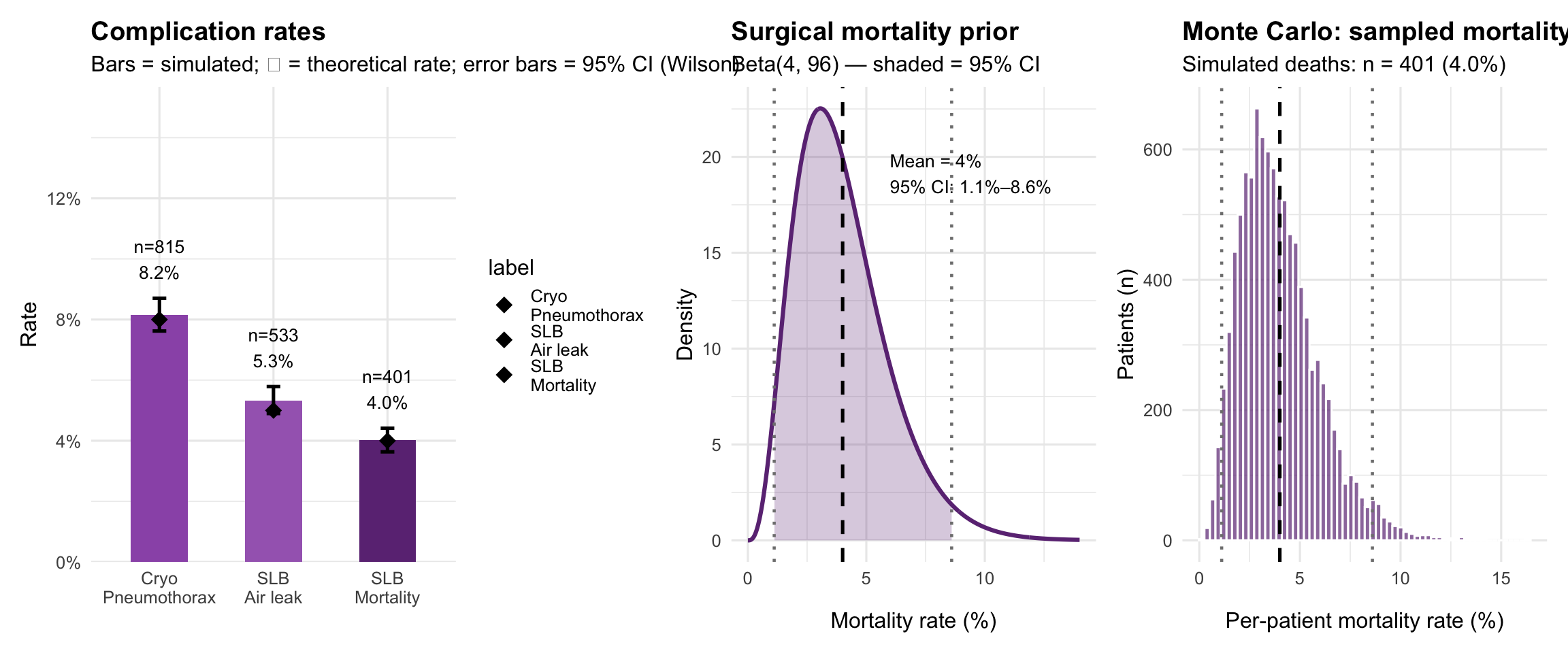
Summary table
sim %>%
  mutate(
    cryo_lbl = cryo_labels[cryo],
    surg_lbl = surg_labels[surg]
  ) %>%
  count(cryo_lbl, surg_lbl) %>%
  group_by(cryo_lbl) %>%
  mutate(pct_group = sprintf("%.1f%%", n / sum(n) * 100)) %>%
  ungroup() %>%
  mutate(pct_total = sprintf("%.1f%%", n / N * 100)) %>%
  rename(
    `Cryo result`          = cryo_lbl,
    `Surgical result`      = surg_lbl,
    `n`                    = n,
    `% in cryo group`      = pct_group,
    `% of total cohort`    = pct_total
  ) %>%
  kbl(caption = "Patient pathways — Monte Carlo simulation (N = 10,000)") %>%
  kable_styling(bootstrap_options = c("striped", "hover", "condensed"),
                full_width = FALSE) %>%
collapse_rows(columns = 1, valign = "top")| Cryo result | Surgical result | n | % in cryo group | % of total cohort |
|---|---|---|---|---|
| High confidence | Concordant | 5738 | 95.2% | 57.4% |
| Discordant – HC other Dx | 137 | 2.3% | 1.4% | |
| Discordant – Unclassifiable | 150 | 2.5% | 1.5% | |
| Low confidence | Concordant | 1853 | 60.0% | 18.5% |
| Discordant – HC other Dx | 639 | 20.7% | 6.4% | |
| Discordant – Unclassifiable | 597 | 19.3% | 6.0% | |
| Noninformative | Concordant | 145 | 16.4% | 1.5% |
| Discordant – HC other Dx | 328 | 37.0% | 3.3% | |
| Discordant – LC other Dx | 413 | 46.6% | 4.1% |
Key findings
sim_final <- sim %>%
  mutate(outcome = if_else(surg == "concordant", "concordant", "discordant"))

n_conc <- sum(sim_final$outcome == "concordant")
n_disc <- sum(sim_final$outcome == "discordant")

cat(sprintf("- **Concordant diagnosis:** %d patients (%.1f%%)\n", n_conc, n_conc/N*100))- Concordant diagnosis: 7736 patients (77.4%)
cat(sprintf("- **Discordant / unclassifiable:** %d patients (%.1f%%)\n", n_disc, n_disc/N*100))- Discordant / unclassifiable: 2264 patients (22.6%)
cat(sprintf("- **Cryobiopsy pneumothorax:** %d patients (%.1f%%)\n", sum(sim$ptx), mean(sim$ptx)*100))- Cryobiopsy pneumothorax: 815 patients (8.2%)
cat(sprintf("- **Surgical mortality:** %d patients (%.1f%%)\n", sum(sim$died), mean(sim$died)*100))- Surgical mortality: 401 patients (4.0%)
cat(sprintf("- **Surgical persistent air leak:** %d patients (%.1f%%)\n", sum(sim$airleak), mean(sim$airleak)*100))- Surgical persistent air leak: 533 patients (5.3%)
Reproducibility:
set.seed(2024)— all results are exactly reproducible.