
Outward Propagation of Freezing from a 1.1 mm Cryoprobe in a Lung Nodule
The problem
An Erbe cryoprobe with an outer diameter of 1.1 mm (radius \(a = 0.55\) mm) and a 3 mm long metal contact tip is advanced into a peripheral lung nodule. The probe is cooled by Joule-Thomson expansion of \(CO_2\); the tip surface falls to roughly \(-80\,^\circ\)C within a second or two. Tissue in contact with the tip freezes, an ice ball grows outward, and when the probe is retracted the adherent frozen tissue is torn out as the biopsy specimen. The size of the sample is limited by the work channel of the bronchoscope, with an internal diameter of 2 mm.
The nodule is 70% water and, as stipulated, is modelled with the thermophysical properties of pure water/ice. The question is how far the freezing front travels, and what shape the frozen mass takes, over freeze times of 1 to 10 s.
Why this is not a simple diffusion problem
Three features make the answer non-obvious, and the third is the one the question specifically asks about.
Latent heat. Freezing water releases 334 kJ/kg. To advance the front by 1 mm the probe must remove roughly 100 times more energy than simply cooling that same water by 1 K. The front is latent-heat limited, not diffusion limited. This is a moving-boundary (Stefan) problem.
Warm-side heat load. The unfrozen tissue sits at 37 \(^\circ\)C and conducts heat toward the front, partly cancelling the cold flux arriving from the probe. The front stops when the two balance.
The insulating effect of the ice itself. All the heat extracted at the freezing front must be conducted back through the shell of ice already formed. In cylindrical geometry the thermal resistance of that shell, per unit length, is
\[R'_{\text{ice}} = \frac{\ln(R/a)}{2\pi k_i}\]
which grows without bound as the front radius \(R\) increases. Ice conducts about 3.7\(\times\) better than water (\(k_i \approx 2.25\) vs \(k_w \approx 0.6\) W m\(^{-1}\)K\(^{-1}\)), so the ice shell is a good conductor in absolute terms - but its resistance still increases logarithmically with thickness, and this is what makes freezing decelerate sharply with time. It is why doubling the freeze time does not double the specimen size.
We handle all three with an enthalpy-method finite-volume solution on an axisymmetric \((r,z)\) grid, and cross-check the radial growth against a closed-form quasi-steady Stefan solution.
Physical parameters
P <- list(
  ## --- water / ice (nodule treated as pure water, as stipulated) -------------
  rho_w = 1000,    c_w = 4180,   k_w = 0.60,   # liquid water, ~37 C
  rho_i = 917,     c_i = 2000,   k_i = 2.25,   # ice, ~-20 C
  Lf    = 334000,                              # latent heat of fusion, J/kg
  Tf    = 0,                                   # equilibrium freezing point, C
  dTmush = 0.5,                                # numerical mushy band width, K
  ## --- boundary / operating conditions --------------------------------------
  Tbody      = 37,      # far-field and initial tissue temperature, C
  Tprobe_min = -80,     # steady-state cryoprobe tip surface temperature, C
  tau_cool   = 0.75,    # e-folding time of tip cool-down, s
  w_perf     = 0,       # Pennes perfusion, kg m^-3 s^-1 (0 = none; see sensitivity)
  c_b        = 3600,    # specific heat of blood, J/kg/K
  k_ice_Tdep = FALSE,   # temperature-dependent ice conductivity?
  latent_scale = 1,     # 1 = pure water; 0.7 = only 70% of mass freezes
  ## --- geometry -------------------------------------------------------------
  a    = 0.55e-3,   # probe radius (1.1 mm OD), m
  Ltip = 3.0e-3,    # length of metal contact tip, m
  ## --- numerics -------------------------------------------------------------
  dx   = 0.055e-3,  # uniform cell size (dr = dz), m -> 10 cells across the radius
  Rmax = 5.0e-3,    # domain radius, m
  zmin = -3.5e-3,   # distal extent of domain (tip apex is z = 0), m
  zmax = 6.0e-3,    # proximal extent of domain, m
  tend = 10,        # simulated freeze time, s
  safety = 0.15     # explicit time-step safety factor
)

data.frame(
  Quantity = c("Density", "Specific heat", "Thermal conductivity",
               "Thermal diffusivity", "Latent heat of fusion",
               "Volumetric latent heat", "Stefan number  c*dT/L  (at -80 C)"),
  Water = c("1000 kg/m3", "4180 J/kg/K", "0.60 W/m/K",
            sprintf("%.2e m2/s", P$k_w/(P$rho_w*P$c_w)), "-", "-", "-"),
  Ice   = c("917 kg/m3", "2000 J/kg/K", "2.25 W/m/K",
            sprintf("%.2e m2/s", P$k_i/(P$rho_i*P$c_i)),
            "334 kJ/kg", "3.34e8 J/m3",
            sprintf("%.2f", P$c_i*80/P$Lf))
) |> kable(caption = "Thermophysical properties used in the simulation.")| Quantity | Water | Ice |
|---|---|---|
| Density | 1000 kg/m3 | 917 kg/m3 |
| Specific heat | 4180 J/kg/K | 2000 J/kg/K |
| Thermal conductivity | 0.60 W/m/K | 2.25 W/m/K |
| Thermal diffusivity | 1.44e-07 m2/s | 1.23e-06 m2/s |
| Latent heat of fusion | - | 334 kJ/kg |
| Volumetric latent heat | - | 3.34e8 J/m3 |
| Stefan number c*dT/L (at -80 C) | - | 0.48 |
#LD15OFFTwo numbers deserve comment.
The thermal diffusivity of ice is 8.5\(\times\) that of water, so once a shell of ice exists the cold penetrates through it quickly; the rate-limiting step is delivering latent heat out of the front, not cooling the ice.
The Stefan number is 0.48, not small. That means the sensible heat needed to chill the ice from 0 \(^\circ\)C down toward the probe temperature is roughly half again the latent heat of freezing it. Classical quasi-steady Stefan solutions that ignore this will overpredict growth substantially - we quantify that below.
Model formulation
Governing equation
We solve the enthalpy form of the heat equation, which handles the moving phase boundary without tracking it explicitly:
\[\frac{\partial H}{\partial t} = \nabla \cdot \left( k(H)\, \nabla T(H) \right) + q_{\text{perf}}\]
where \(H\) is volumetric enthalpy (J m\(^{-3}\)). The constitutive relation \(T(H)\) absorbs the latent heat as a vertical step (smeared over a narrow mushy band \(T_s = -0.5\,^\circ\)C to \(T_l = 0\,^\circ\)C for numerical stability):
\[ T(H) = \begin{cases} H / (\rho_i c_i) & H < H_s \quad \text{(solid)}\\ T_s + (T_l - T_s)\dfrac{H - H_s}{\rho_w L_f} & H_s \le H \le H_l \quad \text{(mushy)}\\ T_l + \dfrac{H - H_l}{\rho_w c_w} & H > H_l \quad \text{(liquid)} \end{cases} \]
with \(H_s = \rho_i c_i T_s\) and \(H_l = H_s + \rho_w L_f\). The liquid fraction \(f = (H - H_s)/(\rho_w L_f)\) clamped to \([0,1]\) sets the local conductivity \(k = k_i + f\,(k_w - k_i)\).
Geometry and boundary conditions
The problem is axisymmetric about the probe axis. Taking \(z = 0\) at the distal apex of the metal tip and increasing \(z\) proximally:
| Region | Location | Treatment |
|---|---|---|
| Metal contact tip | \(r < a\), \(0 \le z \le L_{tip}\) | Dirichlet, \(T = T_p(t)\) |
| Insulated shaft | \(r < a\), \(z > L_{tip}\) | Adiabatic (\(k = 0\)) |
| Tissue | everywhere else | Enthalpy update |
| Far field | \(r = R_{max}\), \(z = z_{min}\), \(z = z_{max}\) | Dirichlet, \(T = 37\,^\circ\)C |
| Axis | \(r = 0\) | Symmetry (zero face area) |
Tissue occupies the region distal to the tip (\(z < 0\)) as well as the annulus around it, so the ice ball can grow forward off the end of the probe as well as sideways. The shaft proximal to the metal tip is insulated, but ice can still creep proximally through the ice itself, and the model captures that.
The tip surface temperature follows an exponential cool-down, \(T_p(t) = T_{body} + (T_{min} - T_{body})(1 - e^{-t/\tau})\) with \(\tau = 0.75\) s, representing the finite time for the Joule-Thomson expansion to bring the tip to its working temperature. This matters a great deal at \(t = 1\) s and hardly at all by \(t = 10\) s; a sensitivity run with an instantaneous step is given later.
We assume perfect thermal contact between metal and tissue (the ice welds itself to the probe - that adhesion is the biopsy mechanism).
Numerical scheme
Explicit finite volume on a uniform cell-centred grid, with exact
cylindrical cell volumes \(V = 2\pi r\,\Delta
r\,\Delta z\) and face areas, harmonic-mean face conductivities
(correct for the sharp \(k\) jump at
the front), and a time step set to a fraction safety of the
2-D explicit stability limit \(\Delta
x^2/(4\alpha_{ice})\).
run_cryo <- function(P, snap_times = seq(0.5, 10, by = 0.5), n_rec = 40) {

  ## ---- grid ---------------------------------------------------------------
  dr <- dz <- P$dx
  Nr <- round(P$Rmax / dr)
  Nz <- round((P$zmax - P$zmin) / dz)
  rc <- (seq_len(Nr) - 0.5) * dr
  zc <- P$zmin + (seq_len(Nz) - 0.5) * dz
  Rm <- matrix(rc, Nr, Nz)
  Zm <- matrix(zc, Nr, Nz, byrow = TRUE)
  Vol <- 2 * pi * Rm * dr * dz

  PROBE <- (Rm < P$a) & (Zm > 0) & (Zm < P$Ltip)
  SHAFT <- (Rm < P$a) & (Zm >= P$Ltip)
  TIS   <- !PROBE & !SHAFT

  ## ---- enthalpy constitutive relation -------------------------------------
  Ts <- P$Tf - P$dTmush; Tl <- P$Tf
  rhoL <- P$rho_w * P$Lf * P$latent_scale
  Hs <- P$rho_i * P$c_i * Ts
  Hl <- Hs + rhoL

  H2T <- function(H) {
    out <- numeric(length(H))
    s <- H < Hs; m <- !s & (H <= Hl); l <- H > Hl
    out[s] <- H[s] / (P$rho_i * P$c_i)
    out[m] <- Ts + (Tl - Ts) * (H[m] - Hs) / rhoL
    out[l] <- Tl + (H[l] - Hl) / (P$rho_w * P$c_w)
    matrix(out, nrow(H), ncol(H))
  }
  H2f <- function(H) matrix(pmin(1, pmax(0, (H - Hs) / rhoL)), nrow(H), ncol(H))

  k_of <- function(f, Tm) {
    ki <- if (P$k_ice_Tdep) pmin(4, P$k_i * 273.15 / pmax(120, 273.15 + Tm)) else P$k_i
    km <- ki + f * (P$k_w - ki)
    km[PROBE] <- 1e4      # metal: forces a Dirichlet condition at the wall face
    km[SHAFT] <- 0        # insulation: no flux
    km
  }
  harm <- function(k1, k2) ifelse(k1 + k2 > 0, 2 * k1 * k2 / (k1 + k2), 0)

  ## ---- geometric face areas (constant) ------------------------------------
  Ar_full <- matrix(2 * pi * (seq_len(Nr) * dr) * dz, Nr, Nz)
  Ar_m <- Ar_full[-Nr, , drop = FALSE]     # internal radial faces
  Az_m <- 2 * pi * Rm[, -Nz, drop = FALSE] * dr   # internal axial faces
  Aout <- Ar_full[Nr, ]                    # outer radial boundary
  Azb  <- 2 * pi * rc * dr                 # axial boundary faces

  ## masks selecting probe-surface faces, for the heat-extraction budget
  mFr <- PROBE[-Nr, , drop = FALSE] & TIS[-1, , drop = FALSE]
  mFz_a <- PROBE[, -Nz, drop = FALSE] & TIS[, -1, drop = FALSE]
  mFz_b <- TIS[, -Nz, drop = FALSE] & PROBE[, -1, drop = FALSE]

  ## ---- time stepping ------------------------------------------------------
  alpha_i <- P$k_i / (P$rho_i * P$c_i)
  dt <- P$safety * dr^2 / alpha_i
  nst <- ceiling(P$tend / dt); dt <- P$tend / nst

  H <- matrix(Hl + P$rho_w * P$c_w * (P$Tbody - Tl), Nr, Nz)
  Tm <- H2T(H); fm <- H2f(H); km <- k_of(fm, Tm)
  E0 <- sum(H[TIS] * Vol[TIS])

  jmid <- which.min(abs(zc - P$Ltip / 2))   # mid-tip plane, for the radial front
  snaps <- vector("list", length(snap_times)); isnap <- 1L
  rec <- vector("list", 0); irec <- 0L

  for (n in seq_len(nst)) {
    tn <- n * dt
    Tm[PROBE] <- P$Tbody + (P$Tprobe_min - P$Tbody) * (1 - exp(-tn / P$tau_cool))

    kf  <- harm(km[-Nr, , drop = FALSE], km[-1, , drop = FALSE])
    Fr  <- kf * Ar_m * (Tm[-Nr, , drop = FALSE] - Tm[-1, , drop = FALSE]) / dr
    kfz <- harm(km[, -Nz, drop = FALSE], km[, -1, drop = FALSE])
    Fz  <- kfz * Az_m * (Tm[, -Nz, drop = FALSE] - Tm[, -1, drop = FALSE]) / dz

    Q <- matrix(0, Nr, Nz)
    Q[-Nr, ] <- Q[-Nr, ] - Fr; Q[-1, ] <- Q[-1, ] + Fr
    Q[, -Nz] <- Q[, -Nz] - Fz; Q[, -1] <- Q[, -1] + Fz

    ## far-field Dirichlet faces (half-cell distance)
    Q[Nr, ] <- Q[Nr, ] + km[Nr, ] * Aout * (P$Tbody - Tm[Nr, ]) / (dr / 2)
    Q[, 1]  <- Q[, 1]  + km[, 1]  * Azb  * (P$Tbody - Tm[, 1])  / (dz / 2)
    Q[, Nz] <- Q[, Nz] + km[, Nz] * Azb  * (P$Tbody - Tm[, Nz]) / (dz / 2)

    ## Pennes perfusion, unfrozen tissue only
    if (P$w_perf > 0) {
      Q <- Q + P$w_perf * P$c_b * (P$Tbody - Tm) * Vol * (fm > 0.5)
    }

    H[TIS] <- H[TIS] + dt * Q[TIS] / Vol[TIS]
    Tm <- H2T(H); fm <- H2f(H); km <- k_of(fm, Tm)

    ## ---- recording --------------------------------------------------------
    if (n %% max(1L, round(nst / n_rec)) == 0 || n == nst) {
      irec <- irec + 1L
      ## radial front at the mid-tip plane: search outward through TISSUE cells
      ## only (cells inside the metal are never updated and still carry f = 1)
      idx  <- which(TIS[, jmid])
      frow <- fm[idx, jmid]; rrow <- rc[idx]
      i0 <- which(frow >= 0.5)[1]
      rfront <- if (is.na(i0)) max(rrow) else if (i0 <= 1) P$a else
        rrow[i0 - 1] + (rrow[i0] - rrow[i0 - 1]) *
          (0.5 - frow[i0 - 1]) / (frow[i0] - frow[i0 - 1])
      Vice <- sum((1 - fm[TIS]) * Vol[TIS])
      ## three-way energy split: latent, sensible-in-ice, sensible-in-liquid
      dTi <- pmax(0, Ts - Tm); dTi[!TIS] <- 0
      E_si <- sum((1 - fm) * P$rho_i * P$c_i * dTi * Vol)
      rec[[irec]] <- data.frame(
        t = tn,
        Tprobe = Tm[PROBE][1],
        r_front = rfront,
        V_ice = Vice,
        power = sum(-Fr[mFr]) + sum(-Fz[mFz_a]) + sum(Fz[mFz_b]),
        E_removed = E0 - sum(H[TIS] * Vol[TIS]),
        E_latent  = rhoL * Vice,
        E_sens_ice = E_si
      )
    }
    while (isnap <= length(snap_times) && tn >= snap_times[isnap] - 1e-12) {
      snaps[[isnap]] <- list(t = snap_times[isnap], T = Tm, f = fm)
      isnap <- isnap + 1L
    }
  }

  list(snaps = snaps, ts = bind_rows(rec),
       grid = list(rc = rc, zc = zc, Rm = Rm, Zm = Zm, Vol = Vol,
                   TIS = TIS, PROBE = PROBE, SHAFT = SHAFT, dr = dr, dz = dz),
       P = P, dt = dt, nst = nst)
}
set.seed(1)
t_run <- system.time(sim <- run_cryo(P))
cat(sprintf("Grid %d x %d = %d cells | dt = %.2e s | %d steps | %.0f s wall clock\n",
length(sim$grid$rc), length(sim$grid$zc),
length(sim$grid$rc) * length(sim$grid$zc),
sim$dt, sim$nst, t_run[["elapsed"]]))## Grid 91 x 173 = 15743 cells | dt = 3.70e-04 s | 27038 steps | 37 s wall clockResults
Dimensions of the ice ball, 1-10 s
The frozen mass is measured from the liquid-fraction field: a cell counts as frozen when \(f < 0.5\), i.e. it has crossed the midpoint of the mushy band. Volumes are computed as \(\sum (1-f)\,V\), which is insensitive to that threshold.
ice_metrics <- function(sn, g, P) {
  ice <- g$TIS & (sn$f < 0.5)
  if (!any(ice)) return(NULL)
  rmax <- max(g$Rm[ice]) + g$dr / 2
  zlo  <- min(g$Zm[ice]) - g$dz / 2
  zhi  <- max(g$Zm[ice]) + g$dz / 2
  Vice <- sum((1 - sn$f[g$TIS]) * g$Vol[g$TIS])
  data.frame(
    t          = sn$t,
    D_max      = 2 * rmax * 1e3,
    wall_ice   = (rmax - P$a) * 1e3,
    distal     = -zlo * 1e3,
    proximal   = (zhi - P$Ltip) * 1e3,
    L_axial    = (zhi - zlo) * 1e3,
    V_ice      = Vice * 1e9,
    mass_mg    = Vice * P$rho_w * 1e6,
    A_xsect    = pi * (rmax * 1e3)^2
  )
}

tbl <- bind_rows(lapply(sim$snaps, ice_metrics, g = sim$grid, P = P))
tbl_int <- tbl |> filter(abs(t - round(t)) < 1e-9)
tbl_int |>
transmute(`Freeze time (s)` = t,
`Max diameter (mm)` = round(D_max, 2),
`Ice thickness on wall (mm)` = round(wall_ice, 2),
`Distal projection (mm)` = round(distal, 2),
`Proximal creep (mm)` = round(proximal, 2),
`Total axial length (mm)` = round(L_axial, 2),
`Volume (mm3)` = round(V_ice, 1),
`Mass (mg)` = round(mass_mg, 1),
`Max cross-section (mm2)` = round(A_xsect, 1)) |>
kable(caption = paste("Ice-ball dimensions vs freeze time. 'Distal projection' is",
"how far the ice extends beyond the tip apex; 'proximal creep'",
"is how far it grows back along the insulated shaft."))| Freeze time (s) | Max diameter (mm) | Ice thickness on wall (mm) | Distal projection (mm) | Proximal creep (mm) | Total axial length (mm) | Volume (mm3) | Mass (mg) | Max cross-section (mm2) |
|---|---|---|---|---|---|---|---|---|
| 1 | 1.76 | 0.33 | 0.37 | 0.16 | 3.52 | 4.9 | 4.9 | 2.4 |
| 2 | 2.42 | 0.66 | 0.64 | 0.32 | 3.96 | 12.2 | 12.2 | 4.6 |
| 3 | 2.86 | 0.88 | 0.80 | 0.49 | 4.29 | 18.8 | 18.8 | 6.4 |
| 4 | 3.19 | 1.04 | 0.97 | 0.60 | 4.57 | 24.6 | 24.6 | 8.0 |
| 5 | 3.41 | 1.15 | 1.03 | 0.70 | 4.73 | 30.0 | 30.0 | 9.1 |
| 6 | 3.63 | 1.27 | 1.14 | 0.76 | 4.90 | 34.9 | 34.9 | 10.3 |
| 7 | 3.85 | 1.38 | 1.19 | 0.82 | 5.01 | 39.6 | 39.6 | 11.6 |
| 8 | 3.96 | 1.43 | 1.24 | 0.87 | 5.11 | 44.1 | 44.1 | 12.3 |
| 9 | 4.18 | 1.54 | 1.30 | 0.93 | 5.23 | 48.4 | 48.4 | 13.7 |
| 10 | 4.29 | 1.59 | 1.35 | 0.98 | 5.33 | 52.5 | 52.5 | 14.5 |
The shape of the frozen tissue
The panels below show the \(0\,^\circ\)C isotherm - the outer surface of the biopsy specimen - in longitudinal cross-section, with the probe drawn to scale. The shaft enters from the left; the metal contact tip is the dark segment; tissue lies everywhere outside.
## extract the freezing front as a mirrored longitudinal outline
front_df <- function(sn, g, P) {
  ## Treat the metal tip as part of the body so the 0 C contour comes out as one
  ## outer outline rather than an extra loop around the probe. The shaft is left
  ## unfrozen, so proximal ice creep still shows up correctly.
  fc <- sn$f; fc[g$PROBE] <- 0
  cl <- contourLines(x = g$rc, y = g$zc, z = fc, levels = 0.5)
  if (!length(cl)) return(NULL)
  bind_rows(lapply(seq_along(cl), function(i) {
    d  <- data.frame(r = cl[[i]]$x, z = cl[[i]]$y)
    dr <- d[rev(seq_len(nrow(d))), , drop = FALSE]   # reversed, for the mirror
    rbind(transmute(d,  x = (P$Ltip - z) * 1e3, y =  r * 1e3),
          transmute(dr, x = (P$Ltip - z) * 1e3, y = -r * 1e3)) |>
      mutate(grp = paste0(sn$t, "_", i))
  })) |> mutate(t = sn$t)
}

probe_layer <- function(P, fill_tip = "grey25", fill_shaft = "grey70") {
  a <- P$a * 1e3; L <- P$Ltip * 1e3
  list(
    annotate("rect", xmin = -3.2, xmax = 0, ymin = -a, ymax = a,
             fill = fill_shaft, colour = "grey40", linewidth = 0.3),
    annotate("rect", xmin = 0, xmax = L, ymin = -a, ymax = a,
             fill = fill_tip, colour = "grey20", linewidth = 0.3)
  )
}
fr_int <- bind_rows(lapply(sim$snaps[abs(sapply(sim$snaps, `[[`, "t") -
round(sapply(sim$snaps, `[[`, "t"))) < 1e-9],
front_df, g = sim$grid, P = P))
ggplot(fr_int, aes(x, y, group = grp)) +
geom_polygon(fill = "#9EC9EC", colour = "#12508F", linewidth = 0.6) +
probe_layer(P) +
facet_wrap(~ factor(paste0(t, " s"),
levels = paste0(sort(unique(t)), " s")), ncol = 5) +
coord_fixed(xlim = c(-3.2, 4.6), ylim = c(-2.6, 2.6)) +
labs(title = "Growth of the ice ball on a 1.1 mm cryoprobe with a 3 mm tip",
subtitle = "Longitudinal section; blue = frozen tissue (0 C isotherm). Probe tip dark grey, insulated shaft light grey.",
x = "Axial distance from proximal end of metal tip (mm)",
y = "Radius (mm)") +
theme(strip.text = element_text(face = "bold"))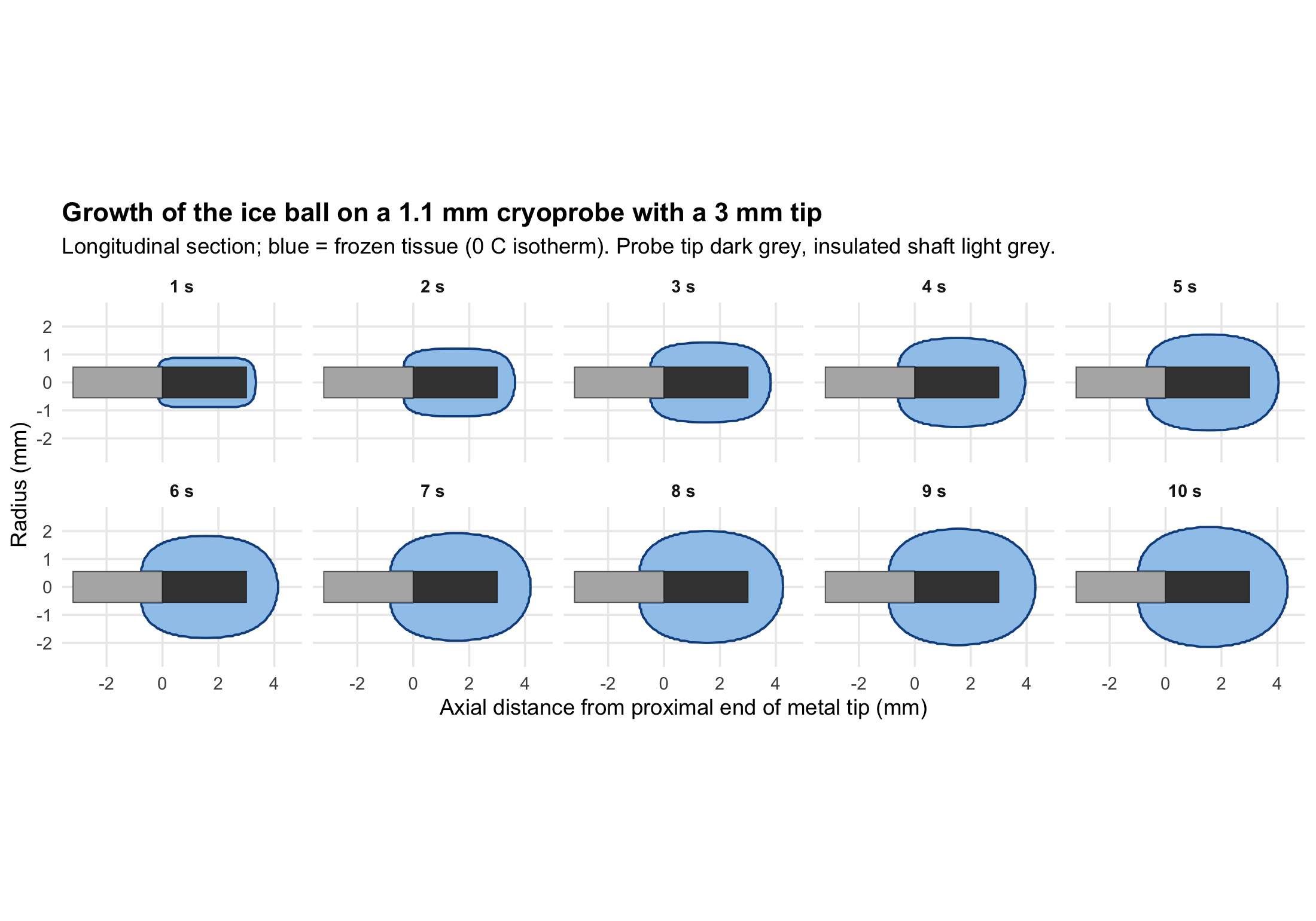
ggplot(fr_int, aes(x, y, group = grp, colour = t)) +
  geom_path(linewidth = 0.75) +
  probe_layer(P) +
  scale_colour_viridis_c(option = "C", end = 0.9, name = "Freeze\ntime (s)",
                         breaks = c(1, 3, 5, 7, 10)) +
  coord_fixed(xlim = c(-3.4, 5.0), ylim = c(-2.8, 2.8)) +
  labs(title = "Nested freezing fronts at 1 s intervals",
       subtitle = "Contour spacing narrows steadily - the signature of the growing ice insulation",
       x = "Axial distance from proximal end of metal tip (mm)", y = "Radius (mm)")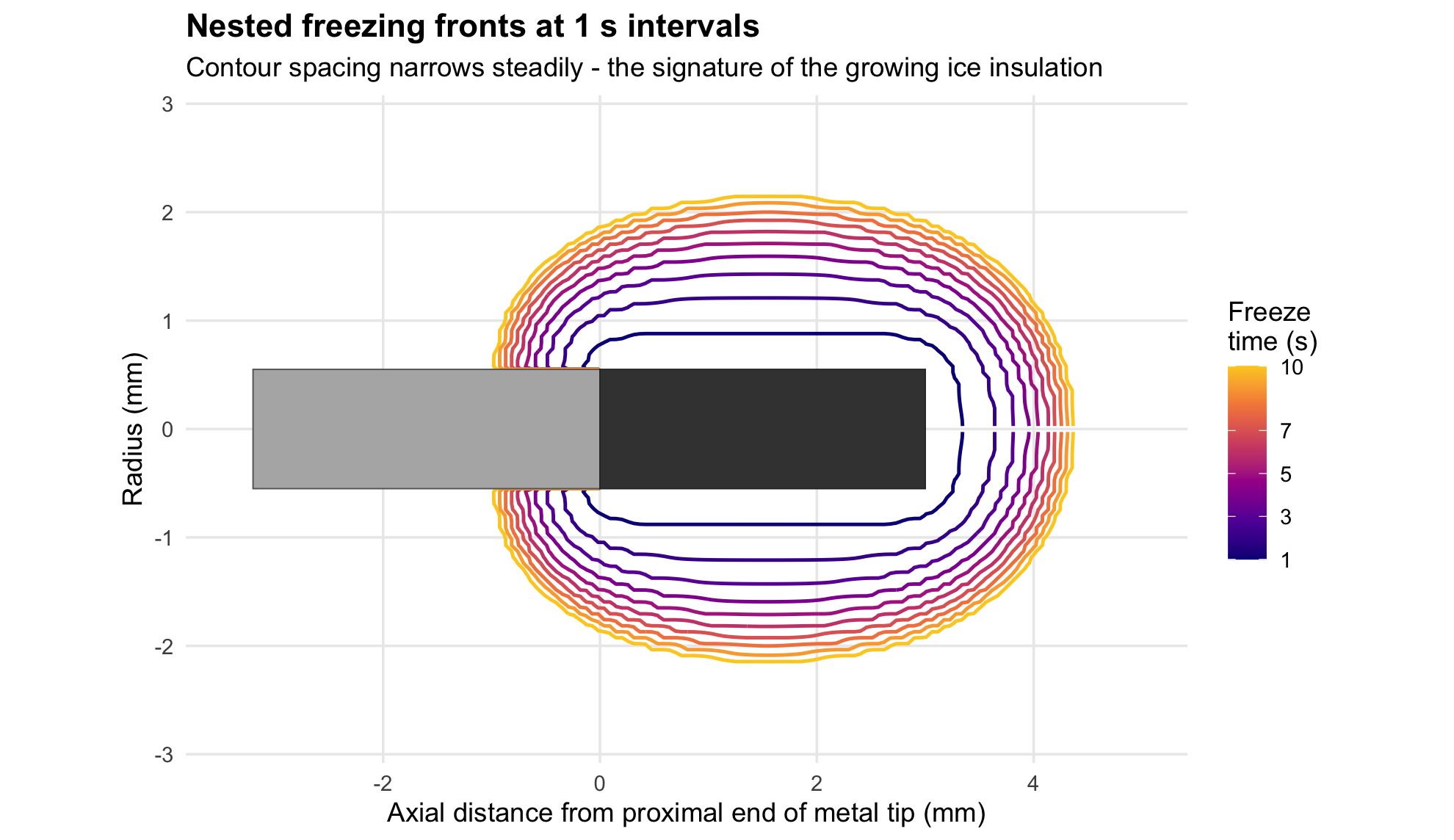
Note the shape. It is not a sphere. Over the first few seconds the ice is a close-fitting cylindrical sleeve on the 3 mm tip - the specimen is elongated, roughly a capsule. As time goes on the ends round off and the mass becomes more ellipsoidal, but even at 10 s it remains longer than it is wide (5.3 mm axially vs 4.3 mm across). The distal cap grows faster than the lateral sleeve because heat there escapes into a three-dimensional hemisphere of cold rather than a two-dimensional annulus.
Temperature field
sn5 <- sim$snaps[[which(sapply(sim$snaps, `[[`, "t") == 5)]]
g <- sim$grid
fld <- expand.grid(r = g$rc, z = g$zc) |>
  mutate(Temp = as.vector(sn5$T),
         inprobe = as.vector(g$PROBE | g$SHAFT),
         x = (P$Ltip - z) * 1e3, y = r * 1e3) |>
  filter(!inprobe)
fld2 <- bind_rows(fld, mutate(fld, y = -y))

ggplot(fld2, aes(x, y, fill = pmax(pmin(Temp, 37), -80))) +
  geom_raster() +
  scale_fill_gradientn(
    colours = c("#08306B", "#2171B5", "#6BAED6", "#C6DBEF", "#FFFFFF",
                "#FEE0D2", "#FC9272", "#CB181D"),
    values  = scales::rescale(c(-80, -60, -40, -20, 0, 10, 25, 37)),
    name = "T (C)", limits = c(-80, 37)) +
  geom_path(data = filter(fr_int, t == 5), aes(x, y, group = grp),
            inherit.aes = FALSE, colour = "black", linewidth = 0.7) +
  probe_layer(P, fill_tip = "grey15", fill_shaft = "grey60") +
  coord_fixed(xlim = c(-3.2, 5.0), ylim = c(-3, 3)) +
  labs(title = "Temperature field at t = 5 s",
       subtitle = "Black line = 0 C isotherm (specimen boundary). Note how tightly the steep gradient hugs the probe.",
       x = "Axial distance from proximal end of metal tip (mm)", y = "Radius (mm)")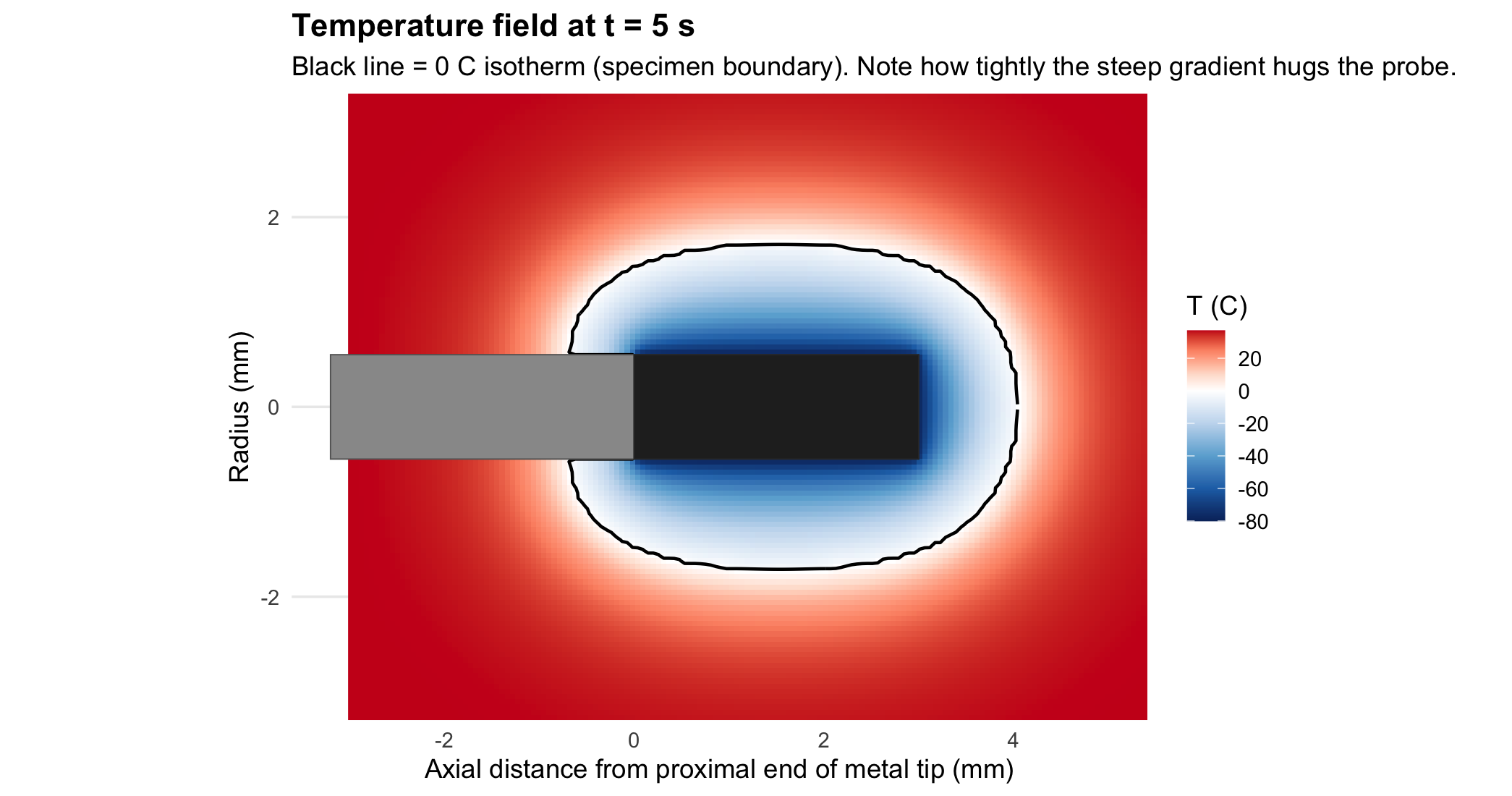
The gradient is extraordinarily steep: the tissue goes from \(-80\,^\circ\)C to \(0\,^\circ\)C across roughly 1.5 mm. Only a thin rind of the specimen ever approaches the lethal \(-20\) to \(-40\,^\circ\)C range; the outer millimetre is barely below freezing. For biopsy this is irrelevant (the tissue is torn out, not ablated), but it is the whole story for cryoablation.
The insulating effect of ice, quantified
Deceleration of the front
ts <- sim$ts |> mutate(r_mm = r_front * 1e3)
## anchor the reference laws at t = 3 s, by which time the tip has reached its
## working temperature; anchoring at 1 s would confound tip cool-down with growth
t_anch <- 3
ref <- ts |> filter(t >= t_anch) |> slice(1)
ts <- ts |> mutate(sqrt_ref = P$a*1e3 + (ref$r_mm - P$a*1e3) * sqrt(t / ref$t),
                   lin_ref  = P$a*1e3 + (ref$r_mm - P$a*1e3) * (t / ref$t))
g10 <- function(v) round(approx(ts$t, v, 10, rule = 2)$y, 2)

ggplot(ts, aes(t, r_mm)) +
  geom_line(aes(y = lin_ref, linetype = "Linear (no insulation)"),
            colour = "grey55") +
  geom_line(aes(y = sqrt_ref, linetype = "sqrt(t) (plain diffusion)"),
            colour = "grey30") +
  geom_line(aes(linetype = "Simulated front"), colour = "#12508F", linewidth = 1.1) +
  geom_vline(xintercept = t_anch, colour = "grey80", linewidth = 0.3) +
  scale_linetype_manual(name = NULL,
    values = c("Simulated front" = "solid",
               "sqrt(t) (plain diffusion)" = "dashed",
               "Linear (no insulation)" = "dotted")) +
  coord_cartesian(ylim = c(0, 4)) +
  labs(title = "Radial position of the freezing front at the mid-tip plane",
       subtitle = "Reference laws anchored to the simulation at t = 3 s, after the tip reaches working temperature",
       x = "Freeze time (s)", y = "Front radius (mm)")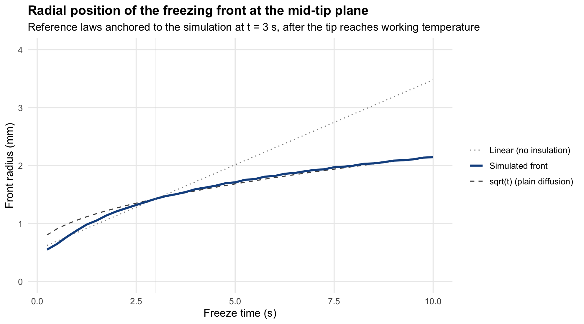
The deceleration is severe. Growth from 1 to 2 s adds 0.33 mm of radius; growth from 9 to 10 s adds only 0.06 mm - a 82% reduction in front velocity for the same one second of freezing.
Measured against the reference laws, at 10 s the front stands at 2.15 mm, against 2.15 mm for the anchored \(\sqrt{t}\) law and 3.48 mm for a front that simply kept its 3 s velocity. Two things are worth separating here. The gap to the linear curve is the insulating effect in its rawest form: a front that never slowed would have reached nearly twice the radius. The near-coincidence with the \(\sqrt{t}\) curve is not evidence against insulation - \(\sqrt{t}\) is the signature of a resistance-limited front, the classical planar Stefan scaling, in which the shell thickness itself sets the rate. Over this particular 3-10 s window the cylindrical \(\ln(R/a)\) correction and the receding warm-side load happen to very nearly cancel, and the two curves are indistinguishable; the agreement is a coincidence of this geometry and time range, not a general law. Before 3 s the simulation runs above the reference only because the tip is still cooling down.
Where the resistance comes from
res <- ts |> filter(!is.na(r_mm), r_mm > P$a*1e3) |>
  mutate(R_ice = log((r_mm/1e3) / P$a) / (2*pi*P$k_i),
         R_ice_rel = R_ice / first(R_ice))

p1 <- ggplot(res, aes(t, R_ice)) +
  geom_line(colour = "#12508F", linewidth = 1) +
  labs(title = "Thermal resistance of the ice shell",
       subtitle = expression(R*minute[ice] == ln(R/a) / (2*pi*k[i])),
       x = "Freeze time (s)", y = "m K / W  (per metre of probe)")

p2 <- ggplot(ts, aes(t, power)) +
  geom_line(colour = "#B2182B", linewidth = 1) +
  labs(title = "Heat extraction rate through the probe surface",
       subtitle = "Start-up spike as the wall first chills, then steady decay as the ice thickens",
       x = "Freeze time (s)", y = "Power (W)")

if (requireNamespace("patchwork", quietly = TRUE)) {
  library(patchwork); p1 + p2
} else { print(p1); print(p2) }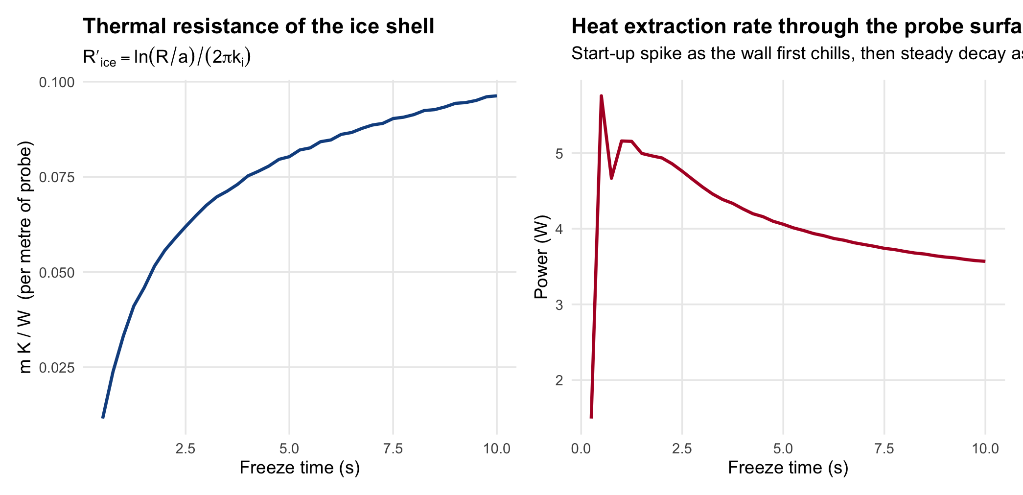
The two panels are the mechanism in full. The ice-shell resistance climbs monotonically; the heat the probe can pull out peaks early (once the tip is cold) and then falls steadily, even though the tip temperature is constant after about 2 s. Nothing about the probe changes - the ice is throttling it.
Where the extracted energy goes
lv <- c("Latent heat of fusion",
        "Sensible: chilling ice below 0 C",
        "Sensible: pre-cooling tissue to 0 C")
en <- ts |> transmute(
    t,
    `Latent heat of fusion`               = E_latent,
    `Sensible: chilling ice below 0 C`    = E_sens_ice,
    `Sensible: pre-cooling tissue to 0 C` = pmax(0, E_removed - E_latent - E_sens_ice)) |>
  pivot_longer(-t, names_to = "Component", values_to = "J") |>
  mutate(Component = factor(Component, levels = lv))

ggplot(en, aes(t, J, fill = Component)) +
  geom_area() +
  scale_fill_manual(values = setNames(c("#4A90D9", "#7FC7A4", "#F0AD4E"), lv)) +
  labs(title = "Cumulative energy budget of the freeze",
       subtitle = "Only the blue band represents new ice being made",
       x = "Freeze time (s)", y = "Energy removed (J)") +
  theme(legend.position = "right")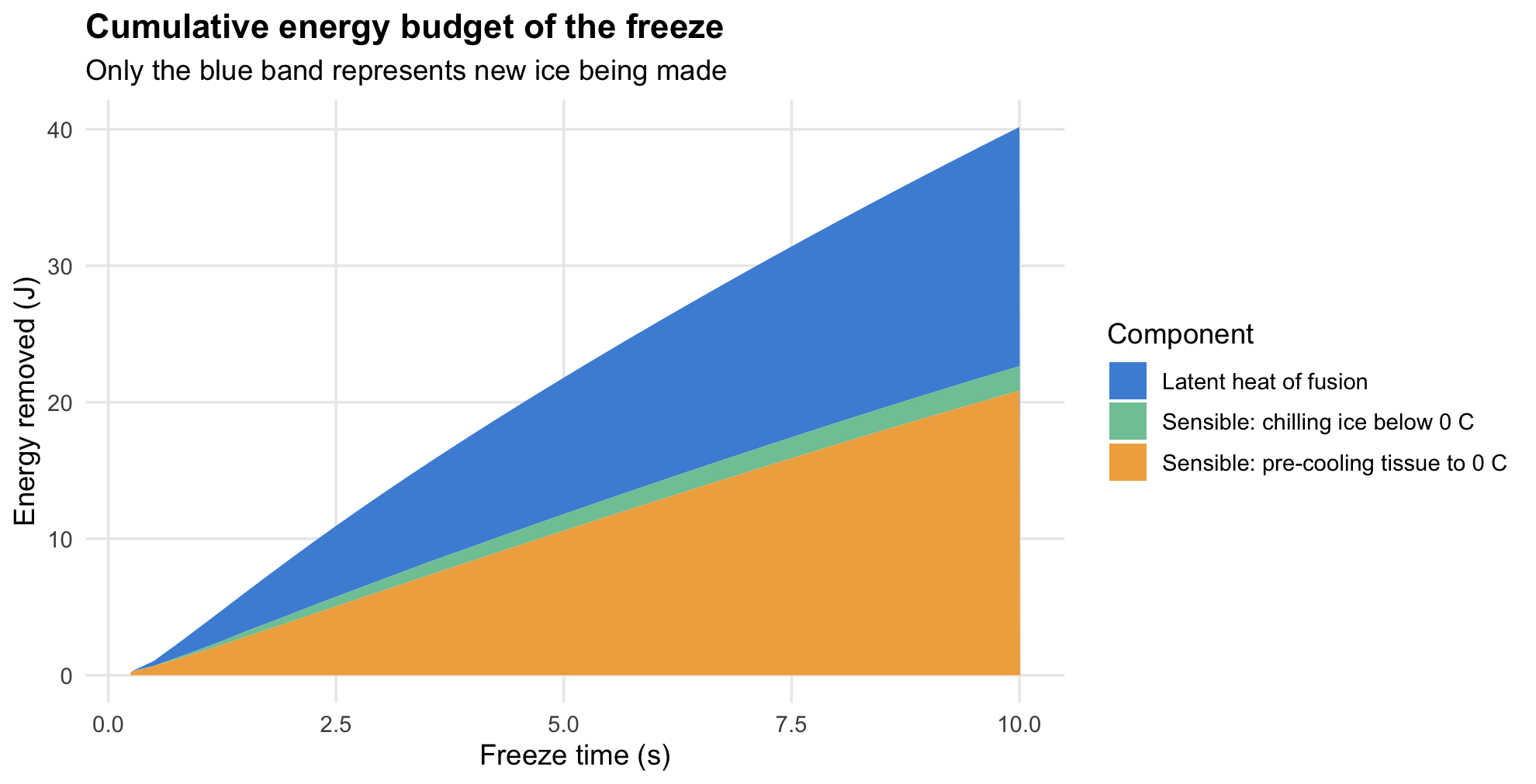
at  <- c(1, 3, 5, 10)
ip  <- function(y) approx(ts$t, y, at, rule = 2)$y
tot <- ip(ts$E_removed); lat <- ip(ts$E_latent); sic <- ip(ts$E_sens_ice)
esp <- data.frame(
  `t (s)`                 = at,
  `Total removed (J)`     = round(tot, 2),
  `Latent (J)`            = round(lat, 2),
  `Sensible, ice (J)`     = round(sic, 2),
  `Sensible, pre-cool (J)`= round(tot - lat - sic, 2),
  `% latent`              = round(100 * lat / tot),
  check.names = FALSE)
kable(esp, caption = "Only part of the cryoprobe's work goes into making new ice.")| t (s) | Total removed (J) | Latent (J) | Sensible, ice (J) | Sensible, pre-cool (J) | % latent |
|---|---|---|---|---|---|
| 1 | 3.50 | 1.62 | 0.19 | 1.69 | 46 |
| 3 | 13.26 | 6.26 | 0.83 | 6.16 | 47 |
| 5 | 21.81 | 10.00 | 1.22 | 10.59 | 46 |
| 10 | 40.16 | 17.53 | 1.79 | 20.85 | 44 |
Less than half of everything the probe extracts actually goes into making new ice. The rest is sensible heat: pre-cooling tissue from 37 \(^\circ\)C down to the freezing point before it can freeze, and then chilling the resulting ice on down toward \(-80\,^\circ\)C. Neither enlarges the specimen. The ice-chilling share is the Stefan number 0.48 showing up as a direct efficiency penalty, and it grows as the freeze goes on, because there is steadily more cold ice to keep cold. This is a second, distinct reason - independent of the conduction resistance above - why long freezes give diminishing returns.
Comparison with the classical quasi-steady Stefan solution
Neglecting the warm-side heat load and treating conduction through the ice as quasi-steady, the cylindrical Stefan problem integrates in closed form:
\[k_i \,\Delta T \, t \;=\; \rho L_{\text{eff}} \left[ \frac{R^2}{2}\ln\frac{R}{a} - \frac{R^2}{4} + \frac{a^2}{4} \right]\]
where \(L_{\text{eff}} = L_f + c_i \Delta T / 2\) crudely accounts for sensible heat in the ice.
analytic_R <- function(t, P, use_Leff = TRUE) {
  dT <- P$Tf - P$Tprobe_min
  Leff <- if (use_Leff) P$Lf + P$c_i * dT / 2 else P$Lf
  sapply(t, function(tt) {
    if (tt <= 0) return(P$a)
    f <- function(R) P$rho_w * Leff *
      (R^2/2 * log(R/P$a) - R^2/4 + P$a^2/4) - P$k_i * dT * tt
    uniroot(f, c(P$a * 1.000001, 0.05))$root
  })
}
tt <- seq(0.05, 10, by = 0.05)
ana <- data.frame(t = tt,
                  `Stefan, latent heat only` = analytic_R(tt, P, FALSE) * 1e3,
                  `Stefan, + sensible correction` = analytic_R(tt, P, TRUE) * 1e3,
                  check.names = FALSE) |>
  pivot_longer(-t, names_to = "Model", values_to = "r_mm")

ggplot() +
  geom_line(data = ana, aes(t, r_mm, colour = Model), linewidth = 0.9) +
  geom_line(data = ts, aes(t, r_mm, colour = "Full 2-D enthalpy simulation"),
            linewidth = 1.2) +
  scale_colour_manual(name = NULL,
    values = c("Stefan, latent heat only" = "#D6604D",
               "Stefan, + sensible correction" = "#F0AD4E",
               "Full 2-D enthalpy simulation" = "#12508F")) +
  coord_cartesian(ylim = c(0, 6)) +
  labs(title = "Closed-form Stefan solutions vs the full simulation",
       subtitle = "The analytic forms omit the 37 C warm-side load, the finite tip cool-down, and axial spreading",
       x = "Freeze time (s)", y = "Front radius (mm)")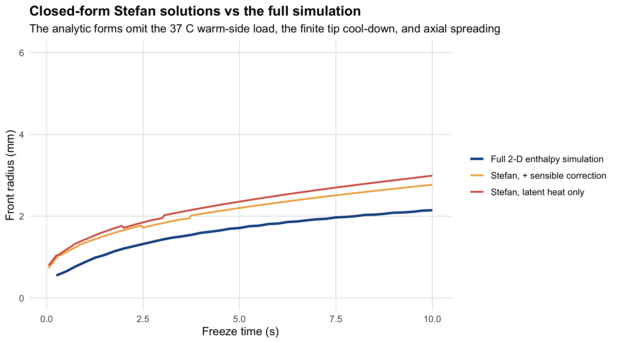
The idealised solution overpredicts by a wide margin, and correcting for sensible heat in the ice recovers a good part of the gap. The residual difference is the warm-side conduction load, the finite tip cool-down, and axial loss of cold into the distal cap - all of which the 2-D model carries and the 1-D analytic form cannot. The analytic curve is useful for scaling intuition (\(R \sim \sqrt{t/\ln R}\)), not for prediction.
Numerical verification
Pc <- modifyList(P, list(dx = 0.110e-3))
sim_c <- run_cryo(Pc, snap_times = 1:10)
tbl_c <- bind_rows(lapply(sim_c$snaps, ice_metrics, g = sim_c$grid, P = Pc))

data.frame(
  `t (s)` = tbl_int$t,
  `V, dx=0.110 mm` = round(tbl_c$V_ice, 1),
  `V, dx=0.055 mm` = round(tbl_int$V_ice, 1),
  `diff %` = round(100 * (tbl_int$V_ice - tbl_c$V_ice) / tbl_int$V_ice, 1),
  `D, dx=0.110 mm` = round(tbl_c$D_max, 2),
  `D, dx=0.055 mm` = round(tbl_int$D_max, 2),
  check.names = FALSE
) |> kable(caption = paste("Grid convergence. The coarse grid runs low because it",
                           "resolves the thin early ice layer poorly; by t >= 3 s the",
"gap settles at 4-6%."))| t (s) | V, dx=0.110 mm | V, dx=0.055 mm | diff % | D, dx=0.110 mm | D, dx=0.055 mm |
|---|---|---|---|---|---|
| 1 | 4.2 | 4.9 | 14.0 | 1.76 | 1.76 |
| 2 | 11.2 | 12.2 | 8.3 | 2.42 | 2.42 |
| 3 | 17.6 | 18.8 | 6.3 | 2.86 | 2.86 |
| 4 | 23.2 | 24.6 | 5.6 | 3.08 | 3.19 |
| 5 | 28.4 | 30.0 | 5.1 | 3.30 | 3.41 |
| 6 | 33.3 | 34.9 | 4.8 | 3.52 | 3.63 |
| 7 | 37.9 | 39.6 | 4.5 | 3.74 | 3.85 |
| 8 | 42.3 | 44.1 | 4.0 | 3.96 | 3.96 |
| 9 | 46.4 | 48.4 | 4.0 | 4.18 | 4.18 |
| 10 | 50.4 | 52.5 | 4.0 | 4.18 | 4.29 |
Convergence is monotone from below, and the gap narrows and then plateaus at 4-6% for \(t \ge 3\) s. The staircased probe surface and the smeared mushy interface make the scheme effectively first-order at the boundary, so a Richardson estimate puts the reported fine-grid volumes within roughly 4-5% of the grid-converged answer - comfortably inside the uncertainty of the input parameters themselves. Linear dimensions agree to within one coarse cell (0.11 mm) at every time.
The 14% gap at \(t = 1\) s is the honest exception: the ice layer is then only 0.33 mm thick, or three coarse cells, and the coarse grid cannot resolve it. The 1 s figures should be read as approximate. Cell size for the reported run is 0.055 mm (10 cells across the probe radius) and the time step is 15% of the explicit stability limit.
Sensitivity analysis
The physics above is solid; the inputs carry real uncertainty. These runs use the coarse grid (justified by the convergence table) so the whole set is cheap.
scen <- list(
  `Baseline (-80 C, 0.75 s cool-down)` = list(),
  `Warmer tip (-60 C)`                 = list(Tprobe_min = -60),
  `Colder tip (-89 C)`                 = list(Tprobe_min = -89),
  `Instant cool-down (tau -> 0)`       = list(tau_cool = 1e-4),
  `Slow cool-down (tau = 1.5 s)`       = list(tau_cool = 1.5),
  `With perfusion (0.5 mL/mL/min)`     = list(w_perf = 0.5 / 60 * 1000),
  `k_ice temperature-dependent`        = list(k_ice_Tdep = TRUE),
  `Only 70% of mass freezes`           = list(latent_scale = 0.7)
)

sens <- bind_rows(lapply(names(scen), function(nm) {
  Ps <- modifyList(modifyList(P, list(dx = 0.110e-3)), scen[[nm]])
  s <- run_cryo(Ps, snap_times = c(1, 3, 5, 10), n_rec = 10)
  bind_rows(lapply(s$snaps, ice_metrics, g = s$grid, P = Ps)) |> mutate(scenario = nm)
}))
sens |>
select(scenario, t, D_max, V_ice) |>
pivot_wider(names_from = t, values_from = c(D_max, V_ice)) |>
transmute(Scenario = scenario,
`D 1s` = round(D_max_1, 2), `D 3s` = round(D_max_3, 2),
`D 5s` = round(D_max_5, 2), `D 10s` = round(D_max_10, 2),
`V 1s` = round(V_ice_1, 1), `V 3s` = round(V_ice_3, 1),
`V 5s` = round(V_ice_5, 1), `V 10s` = round(V_ice_10, 1)) |>
kable(caption = "Max ice diameter (mm) and ice volume (mm3). Baseline first.")| Scenario | D 1s | D 3s | D 5s | D 10s | V 1s | V 3s | V 5s | V 10s |
|---|---|---|---|---|---|---|---|---|
| Baseline (-80 C, 0.75 s cool-down) | 1.76 | 2.86 | 3.30 | 4.18 | 4.2 | 17.6 | 28.4 | 50.4 |
| Warmer tip (-60 C) | 1.54 | 2.42 | 3.08 | 3.74 | 2.9 | 13.5 | 22.0 | 38.1 |
| Colder tip (-89 C) | 1.76 | 2.86 | 3.52 | 4.40 | 4.8 | 19.3 | 31.5 | 55.9 |
| Instant cool-down (tau -> 0) | 2.20 | 3.08 | 3.52 | 4.40 | 10.7 | 23.2 | 33.1 | 54.2 |
| Slow cool-down (tau = 1.5 s) | 1.32 | 2.42 | 3.08 | 4.18 | 1.2 | 12.3 | 23.2 | 46.3 |
| With perfusion (0.5 mL/mL/min) | 1.76 | 2.86 | 3.30 | 4.18 | 4.2 | 17.5 | 28.3 | 50.0 |
| k_ice temperature-dependent | 1.76 | 2.86 | 3.52 | 4.40 | 4.5 | 19.6 | 32.5 | 58.7 |
| Only 70% of mass freezes | 1.76 | 2.86 | 3.52 | 4.40 | 4.8 | 20.0 | 32.5 | 57.5 |
ggplot(sens, aes(t, V_ice, colour = scenario)) +
  geom_line(linewidth = 0.9) + geom_point(size = 1.6) +
  scale_colour_brewer(palette = "Dark2", name = NULL) +
  labs(title = "Sensitivity of ice volume to model assumptions",
       x = "Freeze time (s)", y = expression("Ice volume  (mm"^3*")")) +
  theme(legend.position = "right", legend.text = element_text(size = 8.5))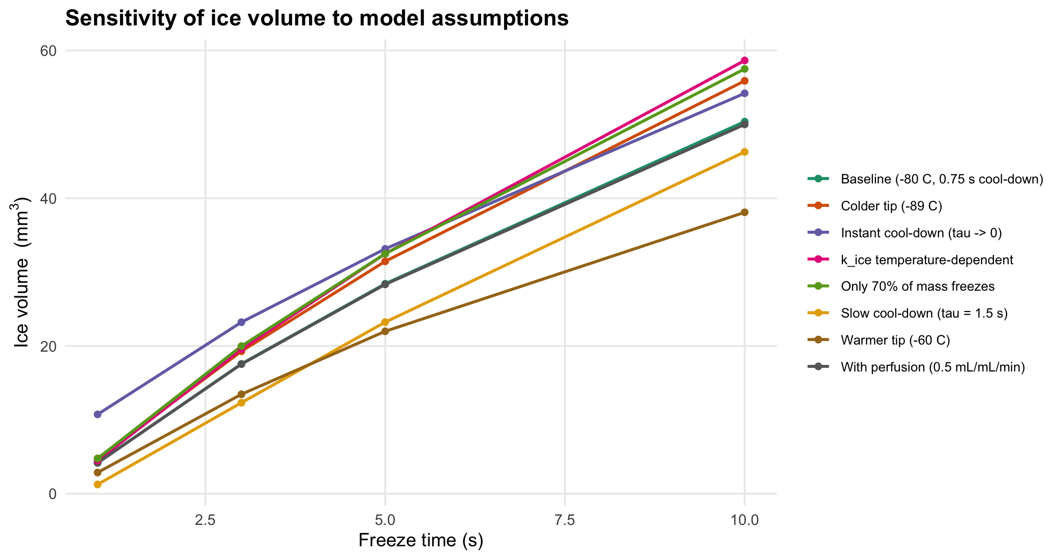
The ordering of effects is worth internalising:
- Tip cool-down time dominates the short freezes. At 1 s the difference between an instantaneous and a 1.5 s cool-down is larger than the difference between a \(-60\,^\circ\)C and a \(-89\,^\circ\)C tip. For 1-3 s freezes, how fast your probe gets cold matters more than how cold it ultimately gets.
- Tip temperature buys volume almost in proportion. Going from \(-60\) to \(-89\,^\circ\)C raises the driving temperature difference by 48% and the 10 s ice volume by 47% - very nearly linear, and only mildly sub-linear at shorter times (about +43% at 3-5 s). A colder probe is a real and near-proportional gain, which is not true of a longer freeze.
- Perfusion is negligible on this timescale. Ten seconds is far shorter than the perfusion time constant, and a nodule is typically poorly perfused anyway. (In a well-perfused organ, or for minute-long ablation freezes, this reverses.)
- Two tissue/ice properties matter about equally, and both point the same way. Letting only 70% of the mass freeze raises the 10 s volume by 14%, and letting ice conductivity rise as it cools (it roughly reaches 3 W m\(^{-1}\)K\(^{-1}\) at \(-80\,^\circ\)C, rather than the constant 2.25 used at baseline) raises it by 16%. Both mean the stipulated pure-water, constant-\(k\) baseline is a conservative choice: a real 70%-water nodule would give a somewhat larger ice ball than the headline numbers above.
Interpretation
Summary of the answer
tbl_int |>
  transmute(`Freeze (s)` = t,
            `Ice ball, D x L (mm)` = sprintf("%.1f x %.1f", D_max, L_axial),
            `Volume (mm3)` = round(V_ice, 1),
            `Mass (mg)` = round(mass_mg, 0),
            `Front velocity (mm/s)` =
              round(c(NA, diff(approx(ts$t, ts$r_mm, t, rule = 2)$y)), 2)) |>
kable(caption = "Headline result: diameter x axial length, and the collapsing front velocity.")| Freeze (s) | Ice ball, D x L (mm) | Volume (mm3) | Mass (mg) | Front velocity (mm/s) |
|---|---|---|---|---|
| 1 | 1.8 x 3.5 | 4.9 | 5 | NA |
| 2 | 2.4 x 4.0 | 12.2 | 12 | 0.33 |
| 3 | 2.9 x 4.3 | 18.8 | 19 | 0.22 |
| 4 | 3.2 x 4.6 | 24.6 | 25 | 0.16 |
| 5 | 3.4 x 4.7 | 30.0 | 30 | 0.12 |
| 6 | 3.6 x 4.9 | 34.9 | 35 | 0.11 |
| 7 | 3.9 x 5.0 | 39.6 | 40 | 0.10 |
| 8 | 4.0 x 5.1 | 44.1 | 44 | 0.08 |
| 9 | 4.2 x 5.2 | 48.4 | 48 | 0.09 |
| 10 | 4.3 x 5.3 | 52.5 | 52 | 0.06 |
For a 1.1 mm Erbe cryoprobe with a 3 mm contact tip in a water-like lung nodule:
- The ice ball reaches roughly 2.9 mm diameter at 3 s and 3.4 mm at 5 s, with an axial length always 1-2 mm greater than its width.
- Returns diminish steeply. Going from 3 s to 6 s roughly 1.9\(\times\) the volume; going from 6 s to 10 s adds only another 50%. Doubling freeze time never doubles the specimen.
- The specimen is a capsule, not a ball - it is the 3 mm tip that sets the shape for the clinically relevant 3-6 s range.
- The ice creeps 0.7-1 mm proximally back over the insulated shaft, purely by conduction through its own ice. This is not a modelling artefact and it slightly increases what has to pass back through the working channel.
What this model does and does not capture
The model is a faithful treatment of the thermal problem, and that is what was asked. Several things stand between its ice ball and a real biopsy specimen, and they all point the same way - the model is an upper bound:
- Ice ball \(\ne\) specimen. The frozen mass is what could come out. What actually detaches is set by where the tissue fails in tension as the probe is withdrawn, which may be inside the ice ball.
- Airway and vessel architecture. A real nodule is not homogeneous. Air-filled alveoli have far lower conductivity and would slow lateral spread markedly; a nearby vessel is a heat source. Modelling the nodule as pure water, as stipulated, ignores both.
- Freezing-point depression. Real tissue freezes over a range of roughly \(-0.5\) to \(-8\,^\circ\)C because of dissolved solutes, not sharply at 0 \(^\circ\)C. This spreads the latent heat over a band and moves the visible boundary inward.
- No contact resistance. Perfect metal-tissue coupling is assumed. Any gap, blood film, or imperfect apposition reduces the result.
- Probe temperature is prescribed, not solved. A real Joule-Thomson probe has finite cooling power; as the ice thickens the tip stays cold, but a probe pushed hard in warm tissue will not hold \(-80\,^\circ\)C perfectly.
The clinically useful conclusion is robust to all of these: the freeze time that matters is the first three or four seconds, and extending a freeze well beyond that costs airway time and bleeding risk to gain progressively less tissue.