
Freezing Propagation in Aerated Lung for Cryobiopsy in DPLD
The problem, and how it differs from a nodule biopsy
In this simulation study, a 1.7 mm Erbe flexible cryoprobe (20402-410) is advanced into the lung periphery to sample parenchyma for diffuse parenchymal lung disease. Unlike in a solid-nodule biopsy, the target is not a water-like mass. It is a two-phase foam: alveolar air plus a thin, continuous network of tissue septa.
That changes the physics in two opposing ways, and the whole analysis turns on which one wins:
- There is far less water to freeze. Latent heat per unit volume scales with the tissue fraction \(f_t\). In fully inflated lung (\(f_t \approx 0.10\)) there is only a tenth as much water per mm\(^3\) as in a solid nodule, so the freezing front should race outward.
- Air is an excellent insulator. \(k_{air} = 0.026\) W m\(^{-1}\)K\(^{-1}\), about 90\(\times\) lower than ice. The effective conductivity of the frozen foam collapses as air fraction rises, which should stall the front.
These effects push in opposite directions and, as we will see, they very nearly cancel - but only under the right model of how a foam conducts heat. Choosing that model is the single most consequential decision in this analysis, so we treat it explicitly rather than burying it.
The probe’s metallic contact tip is 4 mm long. That is a fixed, known input here, which lets the analysis concentrate on the one quantity that is genuinely uncertain: the tissue fraction of the lung being sampled (10% to 60%).
What the literature does and does not provide
Before assuming anything, here is what is actually documented, and what is not.
| Quantity | Value | Used here |
|---|---|---|
| Probe OD | 1.7 | a = 0.85 mm |
| Metallic contact tip length | 4 mm (known) | fixed at 4 mm |
| Tip temperature | -79 C (CO2) | fixed at -79 C |
| Normal lung density, TLC | mean -858 HU -> ~0.14 g/mL -> f_t ~ 14% | included in the f_t sweep |
| Normal lung density, FRC | mean -759 HU -> ~0.24 g/mL -> f_t ~ 24% | BASELINE f_t = 0.24 |
| Effective lung conductivity (in vivo) | 0.16-0.20 W/m/K over the respiratory cycle | used to discriminate mixing models |
| Aerated vs fluid-filled lung | conductivity rises markedly once alveoli fill with fluid | qualitative support for the model choice |
| Clinical specimen size, 1.7 mm probe | median cryobiopsy diameter 6.7 mm (DPLD) | external validation target |
Three points are worth stating upfront.
The tip length is not in the public product literature. Erbe’s product page and the ERBECRYO 2 brochure give diameter and working length only; the 4 mm contact-tip length used throughout is estimated from images of the catheter in the marketing brochure. This matters more than it might appear: tip length sets the length of the frozen capsule almost linearly, so pinning it down removes the dominant geometric uncertainty from every specimen dimension reported below, but errors in the estimate will affect the results.
The 10:90 tissue:air figure corresponds to a fully inflated lung. Quantitative CT of healthy adults gives a mean lung density of \(-858\) HU at total lung capacity and \(-759\) HU at functional residual capacity. Converting with \(\rho \approx (\mathrm{HU}+1000)/1000\) g mL\(^{-1}\) gives tissue fractions of about 14% at TLC and 24% at FRC. Since cryobiopsy is performed on a ventilated patient nearer FRC than TLC, the \(f_t = 0.24\) is used as the baseline and 0.10 as the fully inflated end of the sweep. Both are shown throughout, so nothing hinges on that choice.
The quoted 0.16-0.20 W m\(^{-1}\)K\(^{-1}\) for lung is almost certainly a volume-weighted average, not a measurement. As shown below, a simple parallel mixing rule at FRC reproduces 0.164 W m\(^{-1}\)K\(^{-1}\) almost exactly. That rule is the theoretical upper bound for a two-phase medium and is not physically appropriate for a foam, so the published figure should not be adopted uncritically.
Homogenising the lung: effective properties
We treat the parenchyma as a homogeneous medium whose properties are those of an air/tissue composite with tissue volume fraction \(f_t\). The tissue phase is treated as water/ice, consistent with the previous nodule analysis.
Capacities and latent heat
Air contributes negligible thermal mass: \(f_a \rho_a c_a \approx 1.1 \times 10^3\) J m\(^{-3}\)K\(^{-1}\) against \(f_t \rho_w c_w \approx 1.0 \times 10^6\) J m\(^{-3}\)K\(^{-1}\) even at \(f_t = 0.24\) - about 0.1%. So
\[C_{liq} = f_t \rho_w c_w, \qquad C_{sol} = f_t \rho_i c_i, \qquad (\rho L)_{\text{eff}} = f_t \rho_w L_f\]
The volumetric latent heat scales linearly with tissue fraction. This is exact and model-independent - it is just bookkeeping of how much water is present.
Conductivity: the model that decides everything
Effective conductivity of a two-phase medium is not determined by the volume fractions alone; it depends on the microstructure. We carry three models.
k_air <- 0.026; k_w <- 0.60; k_i <- 2.25

## (1) Bruggeman symmetric effective-medium theory. Random bicontinuous mixture,
##     with a percolation threshold at f = 1/3: below that the conductive phase
##     stops forming an effective backbone and k_eff collapses.
k_emt <- function(ft, ks, ka = k_air) {
  B <- ft*(2*ks - ka) + (1-ft)*(2*ka - ks)
  (B + sqrt(B^2 + 8*ks*ka)) / 4
}
## (2) Maxwell-Eucken with the SOLID as the continuous phase and air as dispersed
##     inclusions. Appropriate when the septal network is structurally continuous.
k_mec <- function(ft, ks, ka = k_air) {
  fa <- 1 - ft
  ks*(2*ks + ka - 2*fa*(ks - ka)) / (2*ks + ka + fa*(ks - ka))
}
## (3) Volume-weighted parallel rule = Wiener upper bound. Physically unattainable
##     for a foam, but it is what much of the tissue-property literature quotes.
k_par <- function(ft, ks, ka = k_air) ft*ks + (1-ft)*ka

mixfun <- function(name) switch(name, emt = k_emt, me = k_mec, par = k_par)| f_tissue | Unfrozen EMT | Unfrozen M-E | Unfrozen par | Frozen EMT | Frozen M-E | Frozen par |
|---|---|---|---|---|---|---|
| 0.100 | 0.035 | 0.066 | 0.083 | 0.036 | 0.180 | 0.248 |
| 0.142 | 0.041 | 0.084 | 0.108 | 0.044 | 0.248 | 0.342 |
| 0.241 | 0.061 | 0.128 | 0.164 | 0.078 | 0.416 | 0.562 |
| 0.400 | 0.130 | 0.205 | 0.256 | 0.325 | 0.713 | 0.916 |
| 0.600 | 0.271 | 0.316 | 0.370 | 0.934 | 1.141 | 1.360 |
| 1.000 | 0.600 | 0.600 | 0.600 | 2.250 | 2.250 | 2.250 |
At the FRC tissue fraction of 0.241 the parallel rule gives 0.164 W m\(^{-1}\)K\(^{-1}\) for unfrozen lung - essentially the 0.16-0.20 range quoted in the literature. This is strong circumstantial evidence that those published values are computed, not measured, and it is why we do not treat them as ground truth.
Which model is right for lung?
This matters enormously, so it deserves an argument rather than an assertion.
EMT is the wrong model here. Bruggeman’s symmetric theory describes a random mixture of two grain populations and has a percolation threshold at \(f = 1/3\): below that fraction the minority phase is assumed to lose its connected backbone and conduction collapses. But alveolar septa are not randomly dispersed grains. They form a fully connected, load-bearing, structurally continuous network that carries the pulmonary capillary bed. That network does not percolation-fail at 20% volume fraction - it is continuous by anatomy. Applying EMT to it imposes a disconnection that does not physically occur.
Maxwell-Eucken with the solid continuous is the appropriate baseline, since it encodes exactly that: a continuous conducting skeleton with non-conducting inclusions. It sits, as it should, between the EMT floor and the parallel ceiling.
We nonetheless carry all three, because the reader should see how much rides on it. The consequence is dramatic:
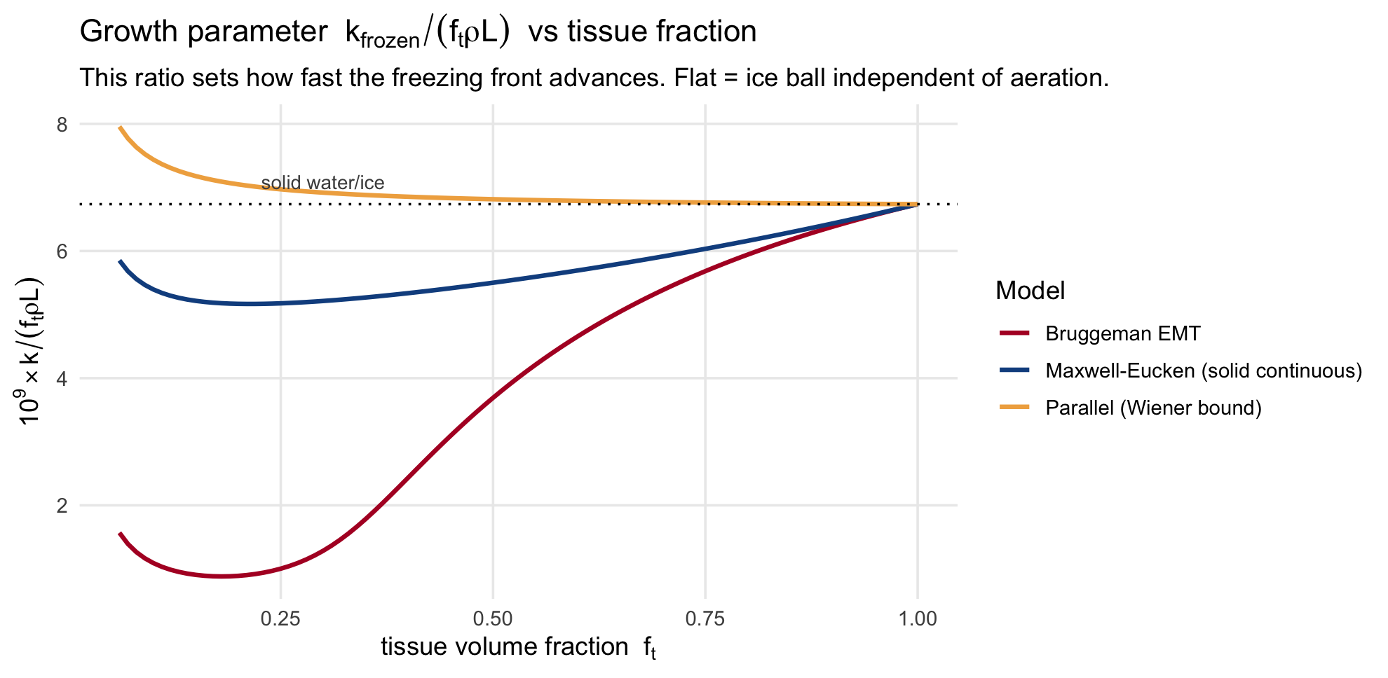
The front speed is governed by \(k_{frozen}/(f_t \rho L)\) - conduction supply divided by latent-heat demand. Under Maxwell-Eucken this ratio is almost flat across the entire physiological range: less water to freeze is almost exactly offset by worse conduction. Under EMT it falls sevenfold below \(f_t \approx 0.35\). So the two models make qualitatively different predictions: one says the ice ball barely cares how aerated the lung is, the other says aeration dominates. We will use the clinical specimen size to decide between them.
Model formulation
Identical to the nodule analysis - a 2-D axisymmetric enthalpy-method Stefan solver - but with composite properties substituted throughout. The probe metal tip is a Dirichlet boundary, the shaft proximal to it is adiabatic, tissue surrounds the tip laterally and distally, and the far field is held at 37 \(^\circ\)C.
P0 <- list(
  rho_w = 1000, c_w = 4180, k_w = 0.60,
  rho_i = 917,  c_i = 2000, k_i = 2.25,
  Lf = 334000, Tf = 0, dTmush = 0.5,
  Tbody = 37, Tprobe_min = -79, tau_cool = 0.75,   # CO2 probe
  w_perf = 0, c_b = 3600, k_ice_Tdep = FALSE,
  ft = 0.241,          # tissue volume fraction (FRC normal lung)
  mix = "me",          # mixing model: "me", "emt" or "par"
  a = 0.85e-3,         # 1.7 mm OD probe
  Ltip = 4.0e-3,       # metallic contact tip length (unpublished; swept 3-5 mm)
  dx = 0.085e-3,       # 10 cells across the probe radius
  Rmax = 8.0e-3, zmin = -5.0e-3, zmax = 12.0e-3,
  tend = 15, safety = 0.15
)
run_cryo <- function(P, snap_times = seq(1, 15, by = 1), n_rec = 60) {
dr <- dz <- P$dx
Nr <- round(P$Rmax / dr); Nz <- round((P$zmax - P$zmin) / dz)
rc <- (seq_len(Nr) - 0.5) * dr
zc <- P$zmin + (seq_len(Nz) - 0.5) * dz
Rm <- matrix(rc, Nr, Nz); Zm <- matrix(zc, Nr, Nz, byrow = TRUE)
Vol <- 2 * pi * Rm * dr * dz
PROBE <- (Rm < P$a) & (Zm > 0) & (Zm < P$Ltip)
SHAFT <- (Rm < P$a) & (Zm >= P$Ltip)
TIS <- !PROBE & !SHAFT
## ---- composite properties ------------------------------------------------
mf <- mixfun(P$mix)
ki_solid <- P$k_i
kF <- mf(P$ft, ki_solid) # frozen composite conductivity
kU <- mf(P$ft, P$k_w) # unfrozen composite conductivity
Cs <- P$ft * P$rho_i * P$c_i # frozen volumetric heat capacity
Cl <- P$ft * P$rho_w * P$c_w # unfrozen volumetric heat capacity
rhoL <- P$ft * P$rho_w * P$Lf # volumetric latent heat
Ts <- P$Tf - P$dTmush; Tl <- P$Tf
Hs <- Cs * Ts; Hl <- Hs + rhoL
H2T <- function(H) {
out <- numeric(length(H))
s <- H < Hs; m <- !s & (H <= Hl); l <- H > Hl
out[s] <- H[s] / Cs
out[m] <- Ts + (Tl - Ts) * (H[m] - Hs) / rhoL
out[l] <- Tl + (H[l] - Hl) / Cl
matrix(out, nrow(H), ncol(H))
}
H2f <- function(H) matrix(pmin(1, pmax(0, (H - Hs) / rhoL)), nrow(H), ncol(H))
k_of <- function(f, Tm) {
kFl <- if (P$k_ice_Tdep)
mf(P$ft, pmin(4, P$k_i * 273.15 / pmax(120, 273.15 + Tm))) else kF
km <- kFl + f * (kU - kFl)
km[PROBE] <- 1e4; km[SHAFT] <- 0
km
}
harm <- function(k1, k2) ifelse(k1 + k2 > 0, 2*k1*k2/(k1+k2), 0)
Ar_full <- matrix(2*pi*(seq_len(Nr)*dr)*dz, Nr, Nz)
Ar_m <- Ar_full[-Nr, , drop = FALSE]
Az_m <- 2*pi*Rm[, -Nz, drop = FALSE]*dr
Aout <- Ar_full[Nr, ]; Azb <- 2*pi*rc*dr
mFr <- PROBE[-Nr, , drop = FALSE] & TIS[-1, , drop = FALSE]
mFz_a <- PROBE[, -Nz, drop = FALSE] & TIS[, -1, drop = FALSE]
mFz_b <- TIS[, -Nz, drop = FALSE] & PROBE[, -1, drop = FALSE]
## stability from whichever phase diffuses fastest in THIS parameter set
alpha_max <- max(kF/Cs, kU/Cl, (if (P$k_ice_Tdep) mf(P$ft, 4)/Cs else 0))
dt <- P$safety * dr^2 / alpha_max
nst <- ceiling(P$tend / dt); dt <- P$tend / nst
H <- matrix(Hl + Cl * (P$Tbody - Tl), Nr, Nz)
Tm <- H2T(H); fm <- H2f(H); km <- k_of(fm, Tm)
E0 <- sum(H[TIS] * Vol[TIS])
jmid <- which.min(abs(zc - P$Ltip/2))
snaps <- vector("list", length(snap_times)); isnap <- 1L
rec <- vector("list", 0); irec <- 0L
for (n in seq_len(nst)) {
tn <- n * dt
Tm[PROBE] <- P$Tbody + (P$Tprobe_min - P$Tbody)*(1 - exp(-tn/P$tau_cool))
kf <- harm(km[-Nr, , drop = FALSE], km[-1, , drop = FALSE])
Fr <- kf * Ar_m * (Tm[-Nr, , drop=FALSE] - Tm[-1, , drop=FALSE]) / dr
kfz <- harm(km[, -Nz, drop = FALSE], km[, -1, drop = FALSE])
Fz <- kfz * Az_m * (Tm[, -Nz, drop=FALSE] - Tm[, -1, drop=FALSE]) / dz
Q <- matrix(0, Nr, Nz)
Q[-Nr, ] <- Q[-Nr, ] - Fr; Q[-1, ] <- Q[-1, ] + Fr
Q[, -Nz] <- Q[, -Nz] - Fz; Q[, -1] <- Q[, -1] + Fz
Q[Nr, ] <- Q[Nr, ] + km[Nr, ]*Aout*(P$Tbody - Tm[Nr, ])/(dr/2)
Q[, 1] <- Q[, 1] + km[, 1] *Azb *(P$Tbody - Tm[, 1]) /(dz/2)
Q[, Nz] <- Q[, Nz] + km[, Nz]*Azb *(P$Tbody - Tm[, Nz])/(dz/2)
if (P$w_perf > 0) Q <- Q + P$w_perf*P$c_b*(P$Tbody - Tm)*Vol*(fm > 0.5)
H[TIS] <- H[TIS] + dt * Q[TIS] / Vol[TIS]
Tm <- H2T(H); fm <- H2f(H); km <- k_of(fm, Tm)
if (n %% max(1L, round(nst/n_rec)) == 0 || n == nst) {
irec <- irec + 1L
idx <- which(TIS[, jmid]); frow <- fm[idx, jmid]; rrow <- rc[idx]
i0 <- which(frow >= 0.5)[1]
rfront <- if (is.na(i0)) max(rrow) else if (i0 <= 1) P$a else
rrow[i0-1] + (rrow[i0]-rrow[i0-1])*(0.5-frow[i0-1])/(frow[i0]-frow[i0-1])
Vice <- sum((1 - fm[TIS]) * Vol[TIS])
dTi <- pmax(0, Ts - Tm); dTi[!TIS] <- 0
rec[[irec]] <- data.frame(
t = tn, r_front = rfront, V_ice = Vice,
power = sum(-Fr[mFr]) + sum(-Fz[mFz_a]) + sum(Fz[mFz_b]),
E_removed = E0 - sum(H[TIS]*Vol[TIS]),
E_latent = rhoL * Vice,
E_sens_ice = sum((1 - fm) * Cs * dTi * Vol))
}
while (isnap <= length(snap_times) && tn >= snap_times[isnap] - 1e-12) {
snaps[[isnap]] <- list(t = snap_times[isnap], T = Tm, f = fm)
isnap <- isnap + 1L
}
}
list(snaps = snaps, ts = bind_rows(rec), P = P, dt = dt, nst = nst,
props = c(kF = kF, kU = kU, Cs = Cs, Cl = Cl, rhoL = rhoL),
grid = list(rc=rc, zc=zc, Rm=Rm, Zm=Zm, Vol=Vol,
TIS=TIS, PROBE=PROBE, SHAFT=SHAFT, dr=dr, dz=dz))
}
ice_metrics <- function(sn, g, P) {
ice <- g$TIS & (sn$f < 0.5)
if (!any(ice)) return(NULL)
rmax <- max(g$Rm[ice]) + g$dr/2
zlo <- min(g$Zm[ice]) - g$dz/2
zhi <- max(g$Zm[ice]) + g$dz/2
Vice <- sum((1 - sn$f[g$TIS]) * g$Vol[g$TIS])
data.frame(t = sn$t,
D_max = 2*rmax*1e3,
wall_ice = (rmax - P$a)*1e3,
distal = -zlo*1e3,
proximal = (zhi - P$Ltip)*1e3,
L_axial = (zhi - zlo)*1e3,
V_ice = Vice*1e9,
tissue_mg = Vice * P$ft * P$rho_w * 1e6,
A_xsect = pi*(rmax*1e3)^2)
}t_run <- system.time(sim <- run_cryo(P0))
cat(sprintf("Baseline: f_t=%.3f (%s), tip=%.1f mm, %d x %d cells, dt=%.2e s, %d steps, %.0f s\n",
P0$ft, P0$mix, P0$Ltip*1e3, length(sim$grid$rc), length(sim$grid$zc),
sim$dt, sim$nst, t_run[["elapsed"]]))## Baseline: f_t=0.241 (me), tip=4.0 mm, 94 x 200 cells, dt=1.15e-03 s, 13039 steps, 24 scat(sprintf("Composite properties: k_frozen=%.3f k_unfrozen=%.3f W/m/K rho*L=%.2e J/m3\n",
sim$props["kF"], sim$props["kU"], sim$props["rhoL"]))## Composite properties: k_frozen=0.416 k_unfrozen=0.128 W/m/K rho*L=8.05e+07 J/m3Baseline result: normal-aeration lung, 4 mm tip
tbl <- bind_rows(lapply(sim$snaps, ice_metrics, g = sim$grid, P = P0))
tbl |> transmute(`Freeze (s)` = t,
                 `Max diameter (mm)` = round(D_max, 2),
                 `Frozen collar on wall (mm)` = round(wall_ice, 2),
                 `Distal projection (mm)` = round(distal, 2),
                 `Proximal creep (mm)` = round(proximal, 2),
                 `Axial length (mm)` = round(L_axial, 2),
                 `Volume (mm3)` = round(V_ice, 1),
                 `Tissue mass (mg)` = round(tissue_mg, 1),
                 `Cross-section (mm2)` = round(A_xsect, 1)) |>
  kable(caption = paste("Frozen specimen vs freeze time. f_t = 0.24 (FRC),",
                        "Maxwell-Eucken, 4 mm tip, -79 C. Note that 'tissue mass'",
"excludes the trapped alveolar air."))| Freeze (s) | Max diameter (mm) | Frozen collar on wall (mm) | Distal projection (mm) | Proximal creep (mm) | Axial length (mm) | Volume (mm3) | Tissue mass (mg) | Cross-section (mm2) |
|---|---|---|---|---|---|---|---|---|
| 1 | 2.21 | 0.26 | 0.32 | 0.10 | 4.42 | 7.6 | 1.8 | 3.8 |
| 2 | 2.89 | 0.60 | 0.58 | 0.27 | 4.85 | 19.2 | 4.6 | 6.6 |
| 3 | 3.23 | 0.77 | 0.83 | 0.44 | 5.27 | 28.5 | 6.9 | 8.2 |
| 4 | 3.57 | 0.94 | 1.00 | 0.52 | 5.52 | 37.0 | 8.9 | 10.0 |
| 5 | 3.91 | 1.10 | 1.09 | 0.61 | 5.70 | 44.8 | 10.8 | 12.0 |
| 6 | 4.08 | 1.19 | 1.17 | 0.69 | 5.86 | 51.8 | 12.5 | 13.1 |
| 7 | 4.25 | 1.28 | 1.26 | 0.78 | 6.04 | 58.3 | 14.1 | 14.2 |
| 8 | 4.42 | 1.36 | 1.34 | 0.78 | 6.12 | 64.6 | 15.6 | 15.3 |
| 9 | 4.59 | 1.45 | 1.34 | 0.86 | 6.20 | 70.6 | 17.0 | 16.5 |
| 10 | 4.76 | 1.53 | 1.43 | 0.95 | 6.38 | 76.4 | 18.4 | 17.8 |
| 11 | 4.93 | 1.62 | 1.51 | 0.95 | 6.46 | 82.0 | 19.8 | 19.1 |
| 12 | 5.10 | 1.70 | 1.51 | 1.03 | 6.54 | 87.3 | 21.0 | 20.4 |
| 13 | 5.10 | 1.70 | 1.60 | 1.03 | 6.63 | 92.5 | 22.3 | 20.4 |
| 14 | 5.27 | 1.79 | 1.60 | 1.03 | 6.63 | 97.7 | 23.5 | 21.8 |
| 15 | 5.44 | 1.87 | 1.68 | 1.12 | 6.80 | 102.6 | 24.7 | 23.2 |
The frozen mass is a foam, not a solid lump of ice. At 15 s the specimen is 103 mm\(^3\) in volume but contains only 25 mg of actual tissue - the rest is trapped air. This is worth holding onto when comparing model output against a pathologist’s measurement of a thawed, partially collapsed specimen.
Shape
front_df <- function(sn, g, P, lab = NULL) {
  fc <- sn$f; fc[g$PROBE] <- 0
  cl <- contourLines(x = g$rc, y = g$zc, z = fc, levels = 0.5)
  if (!length(cl)) return(NULL)
  bind_rows(lapply(seq_along(cl), function(i) {
    d  <- data.frame(r = cl[[i]]$x, z = cl[[i]]$y)
    dd <- d[rev(seq_len(nrow(d))), , drop = FALSE]
    rbind(transmute(d,  x = -z*1e3, y =  r*1e3),
          transmute(dd, x = -z*1e3, y = -r*1e3)) |>
      mutate(grp = paste0(sn$t, "_", i))
  })) |> mutate(t = sn$t, lab = lab %||% "")
}
`%||%` <- function(a, b) if (is.null(a)) b else a

probe_layer <- function(P) {
  a <- P$a*1e3; L <- P$Ltip*1e3
  list(annotate("rect", xmin = -L-4, xmax = -L, ymin = -a, ymax = a,
                fill = "grey70", colour = "grey40", linewidth = 0.3),
       annotate("rect", xmin = -L, xmax = 0, ymin = -a, ymax = a,
                fill = "grey25", colour = "grey15", linewidth = 0.3))
}
show_t <- c(1,2,3,4,5,6,8,10,12,15)
fr <- bind_rows(lapply(sim$snaps[sapply(sim$snaps, `[[`, "t") %in% show_t],
front_df, g = sim$grid, P = P0))
ggplot(fr, aes(x, y, group = grp)) +
geom_polygon(fill = "#9EC9EC", colour = "#12508F", linewidth = 0.55) +
probe_layer(P0) +
facet_wrap(~ factor(paste0(t, " s"), levels = paste0(show_t, " s")), ncol = 5) +
coord_fixed(xlim = c(-8, 4), ylim = c(-3.6, 3.6)) +
labs(title = "Frozen lung attached to a 1.7 mm cryoprobe (4 mm tip, normal aeration)",
subtitle = "Longitudinal section. Distal tip apex at x = 0; probe extends to the left.",
x = "Axial distance from distal tip apex (mm)", y = "Radius (mm)") +
theme(strip.text = element_text(face = "bold"))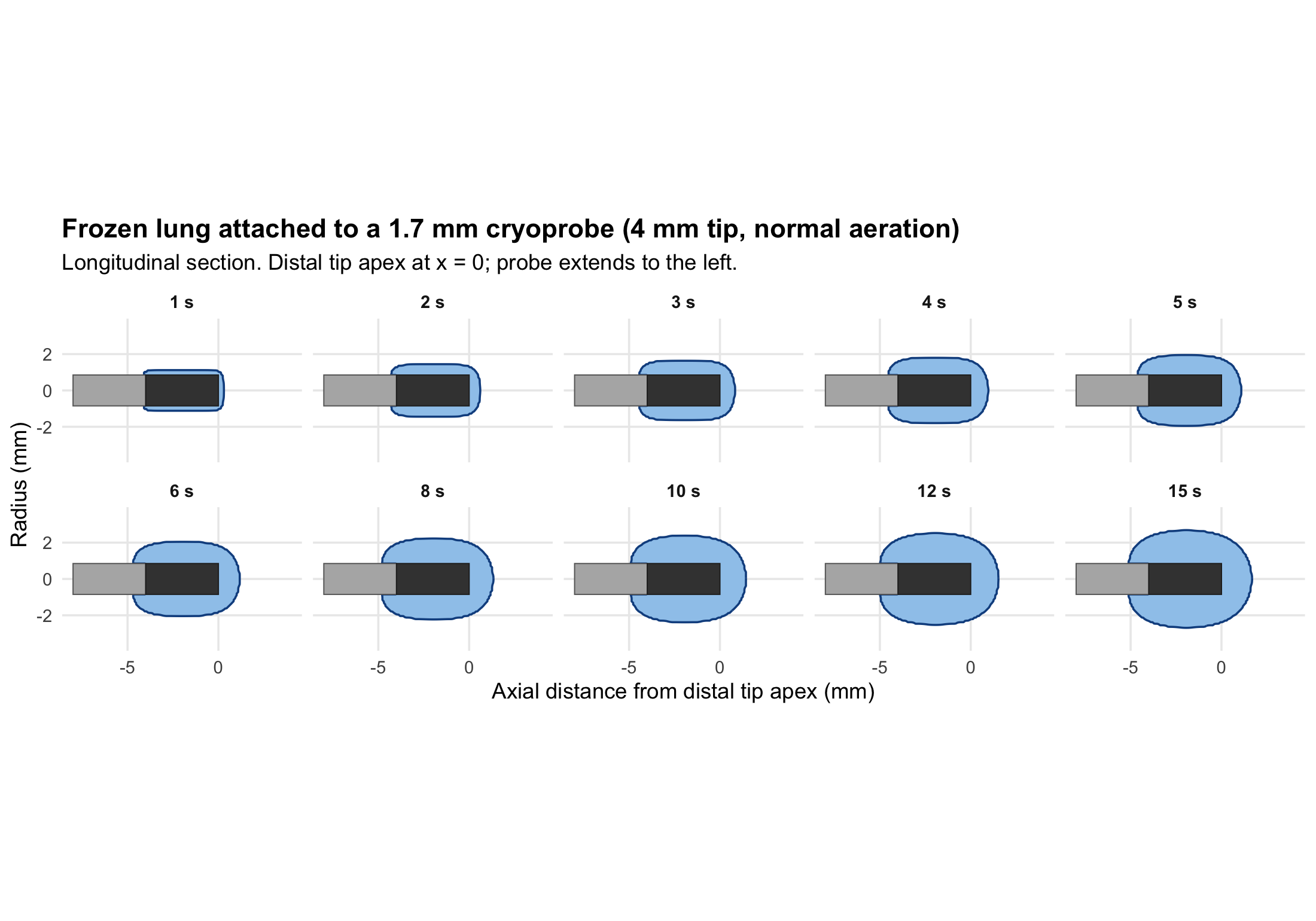
sn6 <- sim$snaps[[which(sapply(sim$snaps, `[[`, "t") == 6)]]
g <- sim$grid
fld <- expand.grid(r = g$rc, z = g$zc) |>
  mutate(Temp = as.vector(sn6$T), inp = as.vector(g$PROBE | g$SHAFT),
         x = -z*1e3, y = r*1e3) |> filter(!inp)
fld <- bind_rows(fld, mutate(fld, y = -y))

ggplot(fld, aes(x, y, fill = pmax(pmin(Temp, 37), -79))) +
  geom_raster() +
  scale_fill_gradientn(
    colours = c("#08306B","#2171B5","#6BAED6","#C6DBEF","#FFFFFF",
                "#FEE0D2","#FC9272","#CB181D"),
    values = scales::rescale(c(-79,-60,-40,-20,0,10,25,37)),
    name = "T (C)", limits = c(-79, 37)) +
  geom_path(data = filter(fr, t == 6), aes(x, y, group = grp),
            inherit.aes = FALSE, colour = "black", linewidth = 0.7) +
  probe_layer(P0) +
  coord_fixed(xlim = c(-8, 4.5), ylim = c(-4, 4)) +
  labs(title = "Temperature field at t = 6 s",
       subtitle = "Black line = 0 C isotherm (specimen boundary)",
       x = "Axial distance from distal tip apex (mm)", y = "Radius (mm)")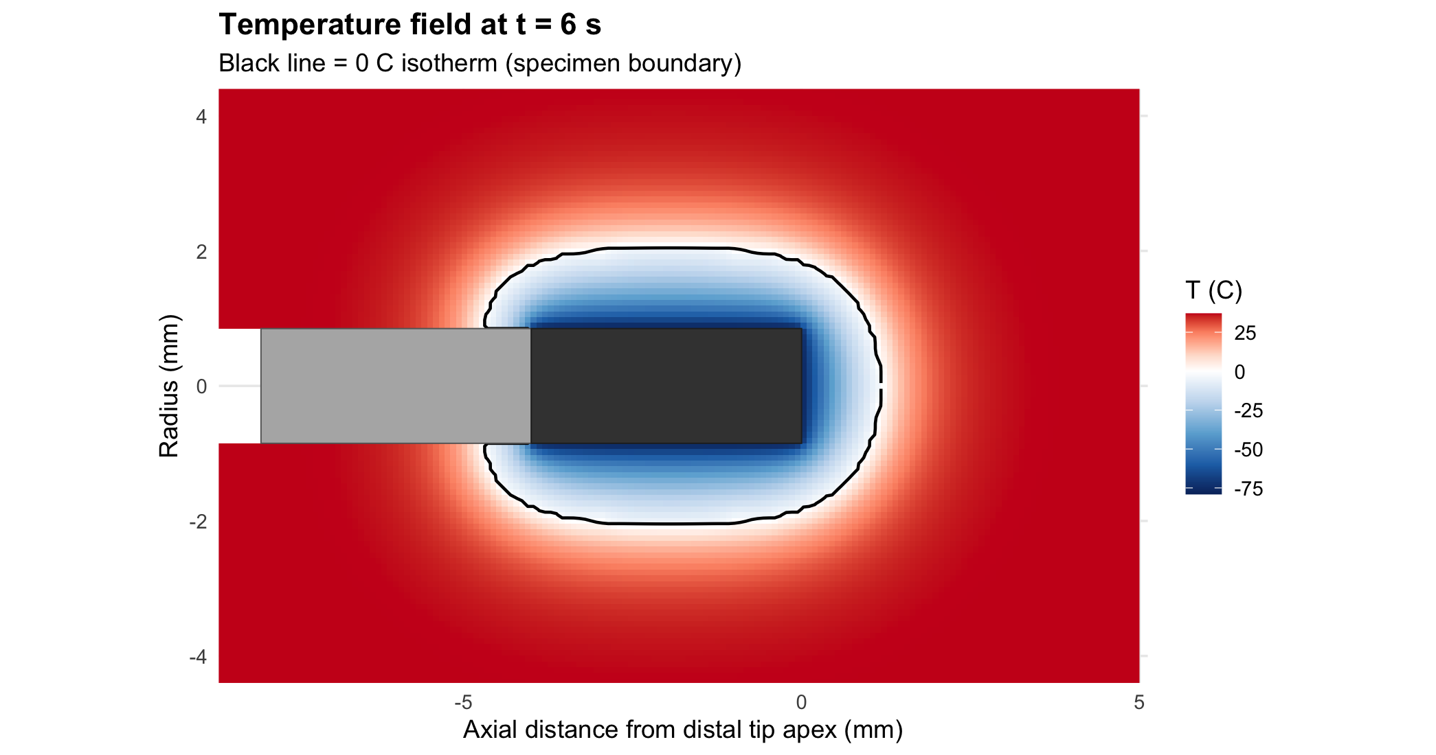
Sensitivity 1: tissue fraction (10% to 60%)
ft_grid <- c(0.10, 0.142, 0.241, 0.40, 0.60)
ft_lab <- c("0.10  fully inflated (your value)", "0.14  normal, TLC",
            "0.24  normal, FRC (baseline)", "0.40  poorly aerated / fibrotic",
            "0.60  dense fibrosis / consolidation")

sweep <- bind_rows(lapply(seq_along(ft_grid), function(i) {
  Pi <- modifyList(P0, list(ft = ft_grid[i], dx = 0.17e-3))
  s <- run_cryo(Pi, snap_times = c(3,5,7,10,15), n_rec = 8)
  bind_rows(lapply(s$snaps, ice_metrics, g = s$grid, P = Pi)) |>
    mutate(ft = ft_grid[i], ftl = ft_lab[i])
}))
sweep |> select(ftl, t, D_max, V_ice, tissue_mg) |>
pivot_wider(names_from = t, values_from = c(D_max, V_ice, tissue_mg)) |>
transmute(`Tissue fraction` = ftl,
`D 5s` = round(D_max_5,1), `D 10s` = round(D_max_10,1),
`D 15s` = round(D_max_15,1),
`V 5s` = round(V_ice_5,1), `V 15s` = round(V_ice_15,1),
`Tissue mg 5s` = round(tissue_mg_5,1),
`Tissue mg 15s` = round(tissue_mg_15,1)) |>
kable(caption = "Effect of aeration, 4 mm tip, Maxwell-Eucken mixing.")| Tissue fraction | D 5s | D 10s | D 15s | V 5s | V 15s | Tissue mg 5s | Tissue mg 15s |
|---|---|---|---|---|---|---|---|
| 0.10 fully inflated (your value) | 3.7 | 4.8 | 5.4 | 42.8 | 98.6 | 4.3 | 9.9 |
| 0.14 normal, TLC | 3.7 | 4.8 | 5.4 | 42.3 | 98.4 | 6.0 | 14.0 |
| 0.24 normal, FRC (baseline) | 3.7 | 4.8 | 5.4 | 42.2 | 99.6 | 10.2 | 24.0 |
| 0.40 poorly aerated / fibrotic | 3.7 | 4.8 | 5.4 | 43.2 | 103.2 | 17.3 | 41.3 |
| 0.60 dense fibrosis / consolidation | 3.7 | 4.8 | 5.4 | 45.4 | 108.6 | 27.2 | 65.2 |
p1 <- ggplot(sweep, aes(t, D_max, colour = factor(ft))) +
  geom_line(linewidth = 1) + geom_point(size = 1.5) +
  scale_colour_viridis_d(option = "D", end = 0.9, name = expression(f[t])) +
  labs(title = "Ice ball diameter barely moves with aeration",
       x = "Freeze time (s)", y = "Max diameter (mm)")
p2 <- ggplot(sweep, aes(t, tissue_mg, colour = factor(ft))) +
  geom_line(linewidth = 1) + geom_point(size = 1.5) +
  scale_colour_viridis_d(option = "D", end = 0.9, name = expression(f[t])) +
  labs(title = "But the tissue actually harvested scales with it",
       x = "Freeze time (s)", y = "Tissue mass (mg)")
if (requireNamespace("patchwork", quietly = TRUE)) {
  p1 + p2 + plot_layout(guides = "collect")
} else { print(p1); print(p2) }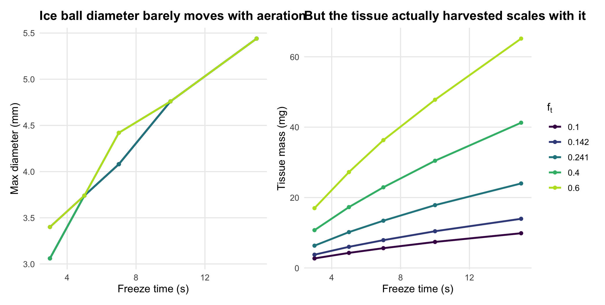
This is the central and most surprising result of the analysis.
The size of the ice ball is remarkably insensitive to how aerated the lung is. Across a sixfold range of tissue fraction the 15 s frozen volume moves only from 98 to 109 mm\(^3\) - about 10% - and the transverse diameter does not change at all at this grid resolution. (Diameters on the coarse sweep grid are quantised in steps of \(2\Delta x = 0.34\) mm, so the continuous volume is the more informative column here.) The reason is the near-cancellation identified earlier: aerated lung has proportionally less water to freeze and proportionally worse conduction, and under a continuous-septal-network model these scale together.
But the diagnostic yield does not follow the ice ball. The tissue mass actually retrieved rises roughly 6.6-fold from fully inflated to densely fibrotic lung, because the same frozen volume contains far more tissue. Clinically this cuts a useful way: for a given freeze time, fibrotic lung yields more diagnostic material than normal lung, at a similar ice-ball size - so the physical size of the frozen mass (which governs the bleeding and pneumothorax risk of tearing it out) does not track the amount of tissue you gain.
Sensitivity 2: the mixing model - the dominant uncertainty
mixes <- c(emt = "Bruggeman EMT", me = "Maxwell-Eucken (baseline)",
           par = "Parallel (Wiener bound)")
mix_sw <- bind_rows(lapply(names(mixes), function(mm)
  bind_rows(lapply(c(0.10, 0.241, 0.60), function(f) {
    Pi <- modifyList(P0, list(mix = mm, ft = f, dx = 0.17e-3))
    s <- run_cryo(Pi, snap_times = c(5, 10, 15), n_rec = 6)
    bind_rows(lapply(s$snaps, ice_metrics, g = s$grid, P = Pi)) |>
      mutate(model = mixes[[mm]], ft = f)
  }))))
mix_sw |> select(model, ft, t, D_max) |>
pivot_wider(names_from = t, values_from = D_max, names_prefix = "D ") |>
transmute(Model = model, `f_t` = ft,
`D 5s` = round(`D 5`,2), `D 10s` = round(`D 10`,2),
`D 15s` = round(`D 15`,2)) |>
kable(caption = paste("Max diameter (mm) by conductivity mixing model. 4 mm tip,",
"-79 C. Coarse grid: diameters are quantised in 0.34 mm steps."))| Model | f_t | D 5s | D 10s | D 15s |
|---|---|---|---|---|
| Bruggeman EMT | 0.100 | 2.72 | 3.06 | 3.40 |
| Bruggeman EMT | 0.241 | 2.72 | 3.06 | 3.40 |
| Bruggeman EMT | 0.600 | 3.74 | 4.42 | 5.10 |
| Maxwell-Eucken (baseline) | 0.100 | 3.74 | 4.76 | 5.44 |
| Maxwell-Eucken (baseline) | 0.241 | 3.74 | 4.76 | 5.44 |
| Maxwell-Eucken (baseline) | 0.600 | 3.74 | 4.76 | 5.44 |
| Parallel (Wiener bound) | 0.100 | 4.08 | 5.10 | 5.78 |
| Parallel (Wiener bound) | 0.241 | 4.08 | 5.10 | 5.78 |
| Parallel (Wiener bound) | 0.600 | 4.08 | 5.10 | 5.78 |
ggplot(mix_sw, aes(t, D_max, colour = model, linetype = factor(ft))) +
  geom_line(linewidth = 0.9) + geom_point(size = 1.4) +
  scale_colour_manual(values = c("Bruggeman EMT" = "#B2182B",
                                 "Maxwell-Eucken (baseline)" = "#12508F",
                                 "Parallel (Wiener bound)" = "#F0AD4E"),
                      name = NULL) +
  scale_linetype_manual(values = c("dotted","solid","dashed"),
                        name = expression(f[t])) +
  labs(title = "The mixing model matters more than every other input combined",
       subtitle = "EMT predicts a small ice ball in aerated lung; the other two do not",
       x = "Freeze time (s)", y = "Max diameter (mm)")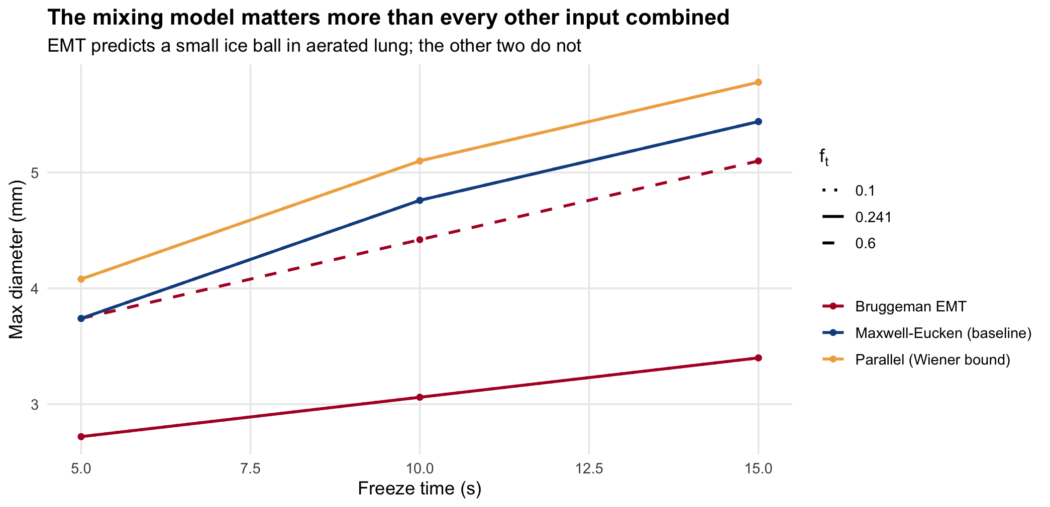
At \(f_t = 0.10\) and 15 s the three models predict diameters of 3.4, 5.4 and 5.8 mm respectively. No other uncertainty in this study comes close to that spread. Any statement about cryobiopsy in aerated lung that does not declare its mixing model is underdetermined.
Using the clinical data to discriminate
Reported transbronchial cryobiopsy with a 1.7 mm probe in DPLD gives a median specimen diameter of 6.7 mm. That is an external, independent constraint - but applying it requires care about which dimension it refers to.
Our specimen is a capsule, markedly longer than it is wide. Pathology reports of cryobiopsy specimens conventionally quote the greatest dimension, which for such a shape is the axial length, not the transverse diameter. We therefore test both readings rather than assume one.
val_runs <- bind_rows(lapply(names(mixes), function(mm) {
  Pi <- modifyList(P0, list(mix = mm, dx = 0.17e-3))
  s <- run_cryo(Pi, snap_times = 1:15, n_rec = 6)
  bind_rows(lapply(s$snaps, ice_metrics, g = s$grid, P = Pi)) |>
    mutate(model = mixes[[mm]])
}))

## first time a monotone series reaches `target`; NA if it never does
cross_t <- function(tt, yy, target) {
  ok <- !is.na(yy); tt <- tt[ok]; yy <- yy[ok]
  if (max(yy) < target) return(NA_real_)
  i <- which(yy >= target)[1]
  if (i == 1) return(tt[1])
  tt[i-1] + (tt[i]-tt[i-1])*(target-yy[i-1])/(yy[i]-yy[i-1])
}
target <- 6.7
val_runs |> group_by(model) |>
summarise(`t to reach 6.7 mm transverse (s)` = round(cross_t(t, D_max, target), 1),
`t to reach 6.7 mm greatest dim (s)` = round(cross_t(t, L_axial, target), 1),
`Transverse D at 15 s (mm)` = round(max(D_max), 1),
`Greatest dim at 15 s (mm)` = round(max(L_axial), 1),
.groups = "drop") |>
kable(caption = paste("Freeze time needed to reach the reported 6.7 mm specimen size,",
"under each reading of 'diameter'. NA = never reached within 15 s.",
"f_t = 0.24."))| model | t to reach 6.7 mm transverse (s) | t to reach 6.7 mm greatest dim (s) | Transverse D at 15 s (mm) | Greatest dim at 15 s (mm) |
|---|---|---|---|---|
| Bruggeman EMT | NA | NA | 3.4 | 5.3 |
| Maxwell-Eucken (baseline) | NA | 14.4 | 5.4 | 6.8 |
| Parallel (Wiener bound) | NA | 10.4 | 5.8 | 7.1 |
val_long <- val_runs |>
  select(model, t, `Transverse diameter` = D_max,
         `Greatest dimension (axial)` = L_axial) |>
  pivot_longer(c(`Transverse diameter`, `Greatest dimension (axial)`),
               names_to = "dim", values_to = "mm")

ggplot(val_long, aes(t, mm, colour = model)) +
  annotate("rect", xmin = 5, xmax = 8, ymin = -Inf, ymax = Inf,
           fill = "grey70", alpha = 0.20) +
  geom_hline(yintercept = target, colour = "black", linewidth = 0.7) +
  geom_line(linewidth = 0.9) +
  facet_wrap(~ dim) +
  scale_colour_manual(values = c("Bruggeman EMT" = "#B2182B",
                                 "Maxwell-Eucken (baseline)" = "#12508F",
                                 "Parallel (Wiener bound)" = "#F0AD4E"), name = NULL) +
  labs(title = "Model predictions against the reported 6.7 mm clinical specimen size",
       subtitle = "1.7 mm probe, 4 mm tip. Black line = reported median; grey band = typical clinical freeze window",
       x = "Freeze time (s)", y = "Specimen dimension (mm)") +
  theme(legend.position = "right")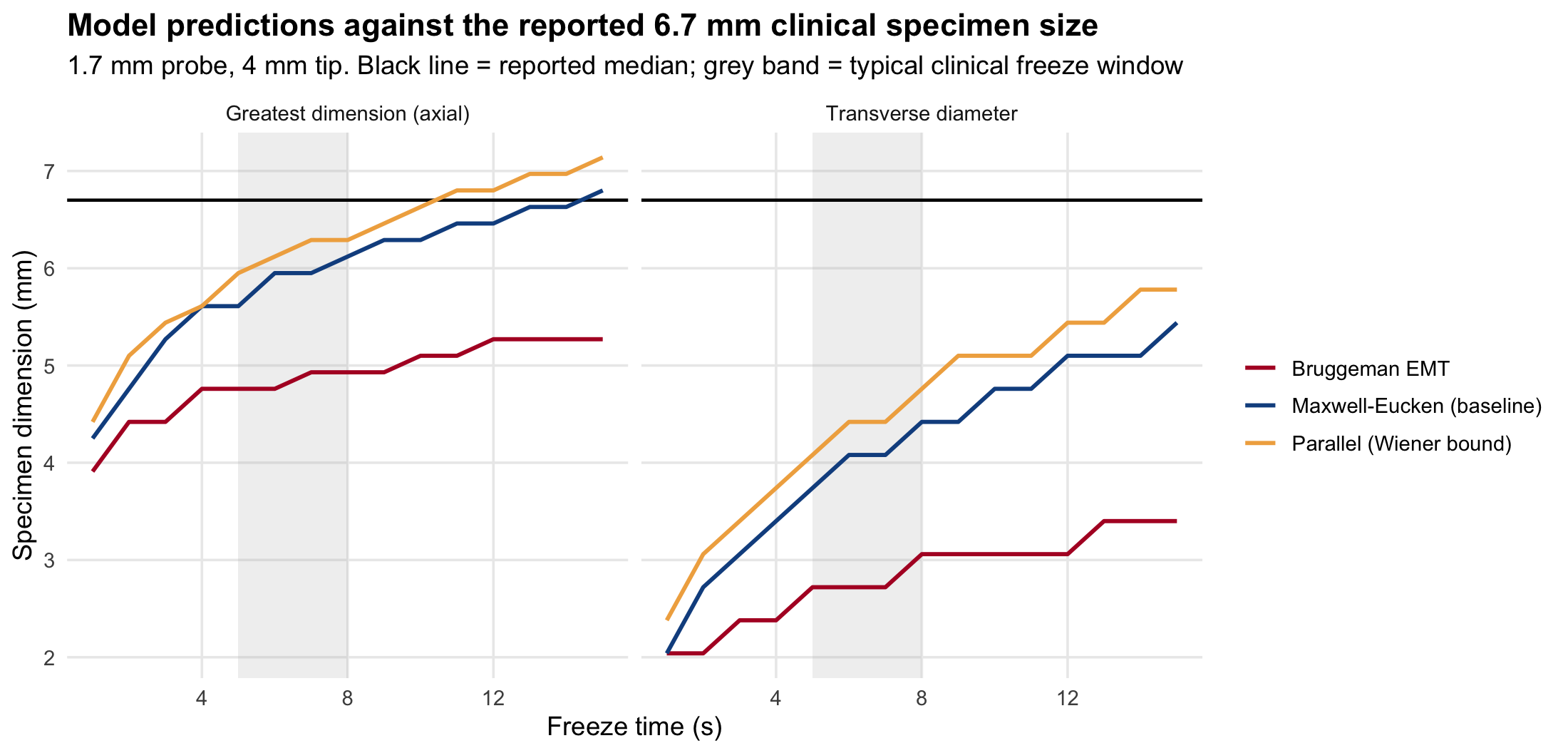
The comparison must be read with care: a frozen ice ball and a fixed, thawed pathology specimen are not the same object, and the ice ball is an upper bound on what detaches. With the tip length now fixed at its true 4 mm, the result is sharper than before - and less comfortable:
- Read as a transverse diameter, no model reaches 6.7 mm within 15 s. The best case is the parallel bound at 5.8 mm, and the baseline Maxwell-Eucken model reaches only 5.4 mm.
- Read as the greatest dimension, the model still falls short at clinical freeze times. Maxwell-Eucken does not reach 6.7 mm until 14.4 s, and the parallel bound not until 10.4 s. At a clinically typical 5-8 s, the predicted greatest dimension is 6.0 mm - roughly 11% short of the reported median.
- Bruggeman EMT remains firmly falsified, reaching only 4.8 mm greatest dimension at 6 s and stalling at 3.4 mm transverse. Since the ice ball is an upper bound on the specimen, this is a genuine falsification.
This is a real and instructive discrepancy, and fixing the tip length is what exposed it. In the earlier version of this analysis the unknown tip length could absorb the gap - a 5 mm tip reconciled the model with the clinical figure at about 5 s. With the tip known to be 4 mm that escape route is closed, and the model under-predicts the reported specimen size at realistic freeze times under every conductivity model tested.
Three explanations are compatible with the physics, and they are not mutually exclusive:
- The specimen is not just the ice ball. Retraction tears tissue, and the fracture need not follow the 0 \(^\circ\)C isotherm. Frozen lung is brittle and welded to surrounding parenchyma; some tissue beyond the frozen margin plausibly comes with it. The model computes the frozen zone, which is a lower bound on what tears even while being an upper bound on what freezes.
- The tissue at the probe is denser than the whole-lung average. Wedging, atelectasis, blood and oedema all raise the local tissue fraction. Note, however, that this does not rescue the size: the ice ball is nearly independent of aeration (see the tissue-fraction sensitivity above), so a denser target yields more tissue at much the same dimensions. Density explains yield, not size.
- The reported dimension may not be measured on a comparable object. A 6.7 mm median is quoted for fixed specimens whose relationship to the frozen mass - collapsed foam, irregular tags, greatest-dimension convention - is not specified.
Explanation 2 is the one that can be excluded on the model’s own evidence, which is a genuinely useful narrowing. The remaining candidates are mechanical and methodological rather than thermal, which is to say: the thermal model is probably not the thing that is wrong here.
The insulating effect of the frozen foam
ts <- sim$ts |> mutate(r_mm = r_front*1e3)
t_anch <- 4
ref <- ts |> filter(t >= t_anch) |> slice(1)
ts <- ts |> mutate(sqrt_ref = P0$a*1e3 + (ref$r_mm - P0$a*1e3)*sqrt(t/ref$t),
                   lin_ref  = P0$a*1e3 + (ref$r_mm - P0$a*1e3)*(t/ref$t))
g15 <- function(v) round(approx(ts$t, v, 15, rule = 2)$y, 2)

ggplot(ts, aes(t, r_mm)) +
  geom_line(aes(y = lin_ref, linetype = "Linear (no insulation)"), colour = "grey55") +
  geom_line(aes(y = sqrt_ref, linetype = "sqrt(t)"), colour = "grey30") +
  geom_line(aes(linetype = "Simulated front"), colour = "#12508F", linewidth = 1.1) +
  geom_vline(xintercept = t_anch, colour = "grey85", linewidth = 0.3) +
  scale_linetype_manual(name = NULL,
    values = c("Simulated front"="solid","sqrt(t)"="dashed",
               "Linear (no insulation)"="dotted")) +
  coord_cartesian(ylim = c(0, 8)) +
  labs(title = "Radial freezing front at the mid-tip plane",
       subtitle = "Reference laws anchored at t = 4 s, after the tip reaches working temperature",
       x = "Freeze time (s)", y = "Front radius (mm)")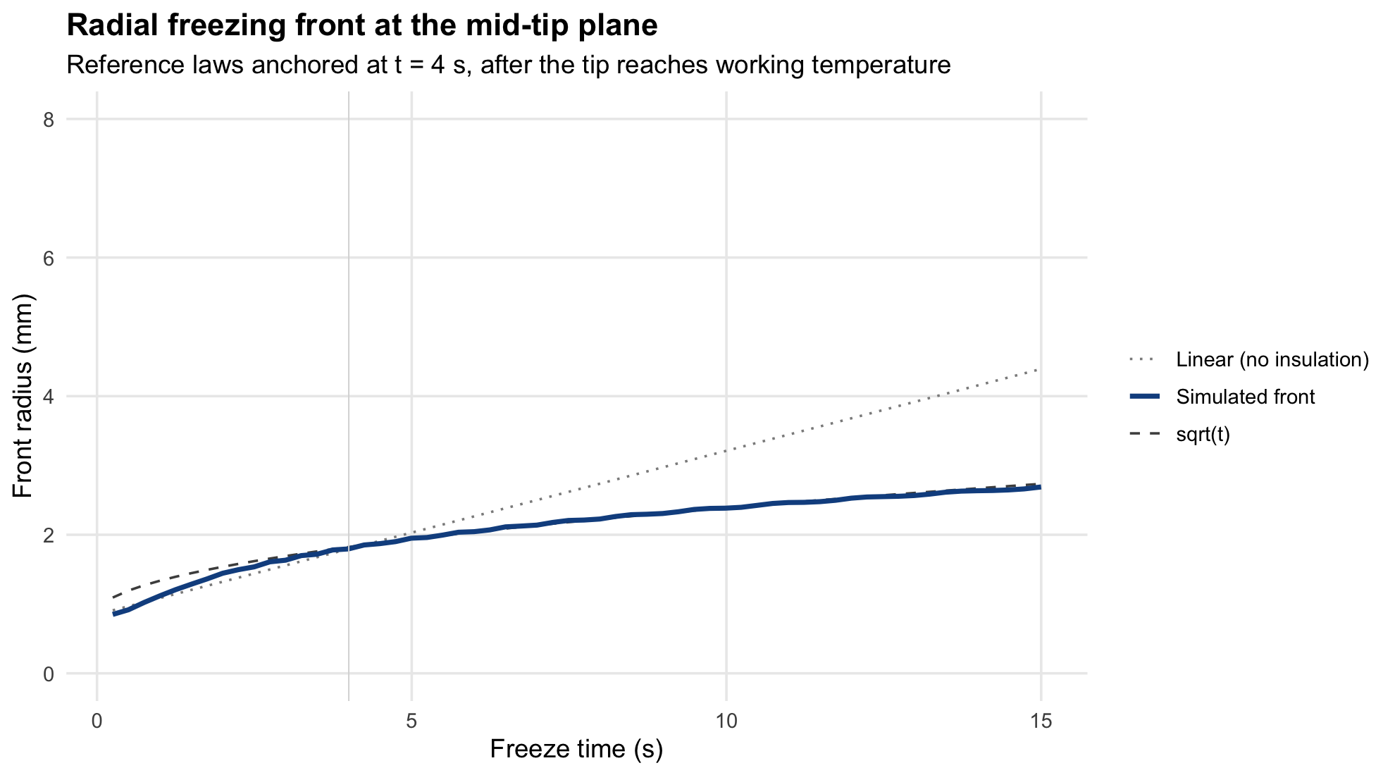
At 15 s the front stands at 2.69 mm against 2.73 mm for the anchored \(\sqrt{t}\) law and 4.39 mm for a front that simply kept its 4 s velocity. Radial growth slows from 0.19 mm/s between 2 and 3 s to 0.05 mm/s between 14 and 15 s.
res <- ts |> filter(r_mm > P0$a*1e3) |>
  mutate(R_ice = log((r_mm/1e3)/P0$a)/(2*pi*sim$props[["kF"]]))
q1 <- ggplot(res, aes(t, R_ice)) + geom_line(colour = "#12508F", linewidth = 1) +
  labs(title = "Thermal resistance of the frozen collar",
       subtitle = expression(ln(R/a)/(2*pi*k[frozen])*"  with the COMPOSITE conductivity"),
       x = "Freeze time (s)", y = "m K / W (per metre)")
q2 <- ggplot(ts, aes(t, power)) + geom_line(colour = "#B2182B", linewidth = 1) +
  labs(title = "Heat extraction rate at the probe surface",
       subtitle = "Start-up spike, then steady decay as the frozen collar thickens",
       x = "Freeze time (s)", y = "Power (W)")
if (requireNamespace("patchwork", quietly = TRUE)) { q1 + q2 } else { print(q1); print(q2) }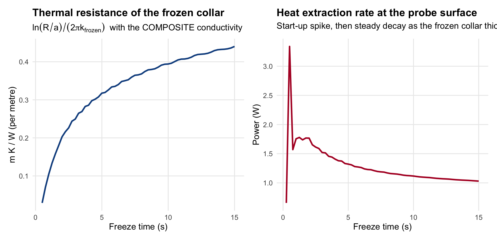
Because the composite conductivity is roughly 5\(\times\) lower than solid ice, the resistance of the frozen collar is correspondingly larger than in the nodule case. The insulating effect is therefore stronger in lung than in a solid nodule - it is just that the latent heat demand falls in step, which is why the net front speed barely changes.
lv <- c("Latent heat of fusion","Sensible: chilling frozen tissue",
        "Sensible: pre-cooling to 0 C")
en <- ts |> transmute(t,
    `Latent heat of fusion` = E_latent,
    `Sensible: chilling frozen tissue` = E_sens_ice,
    `Sensible: pre-cooling to 0 C` = pmax(0, E_removed - E_latent - E_sens_ice)) |>
  pivot_longer(-t, names_to = "Component", values_to = "J") |>
  mutate(Component = factor(Component, levels = lv))
ggplot(en, aes(t, J, fill = Component)) + geom_area() +
  scale_fill_manual(values = setNames(c("#4A90D9","#7FC7A4","#F0AD4E"), lv)) +
  labs(title = "Cumulative energy budget", x = "Freeze time (s)",
       y = "Energy removed (J)") + theme(legend.position = "right")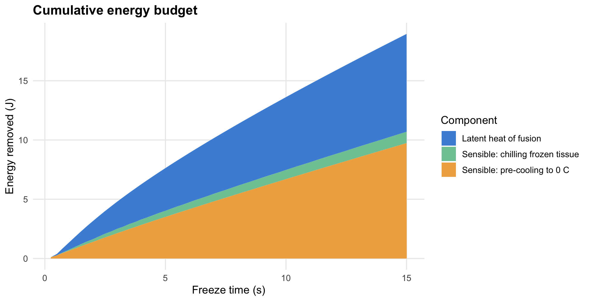
at <- c(3, 5, 10, 15); ip <- function(y) approx(ts$t, y, at, rule = 2)$y
tot <- ip(ts$E_removed); lat <- ip(ts$E_latent); sic <- ip(ts$E_sens_ice)
data.frame(`t (s)` = at, `Total (J)` = round(tot,2), `Latent (J)` = round(lat,2),
           `Sensible, frozen (J)` = round(sic,2),
           `Sensible, pre-cool (J)` = round(tot-lat-sic,2),
           `% latent` = round(100*lat/tot), check.names = FALSE) |>
kable(caption = "Energy budget. Total energies are far smaller than in a solid nodule.")| t (s) | Total (J) | Latent (J) | Sensible, frozen (J) | Sensible, pre-cool (J) | % latent |
|---|---|---|---|---|---|
| 3 | 4.80 | 2.29 | 0.37 | 2.14 | 48 |
| 5 | 7.63 | 3.61 | 0.52 | 3.51 | 47 |
| 10 | 13.62 | 6.15 | 0.78 | 6.70 | 45 |
| 15 | 18.95 | 8.26 | 0.96 | 9.74 | 44 |
The absolute energies are small - a few joules over the whole freeze - because there is so little water present. The probe is not working hard in a thermal sense; it is limited by getting the cold through the insulating frozen foam.
Numerical verification
sim_c <- run_cryo(modifyList(P0, list(dx = 0.17e-3)), snap_times = c(1,3,5,10,15))
tc <- bind_rows(lapply(sim_c$snaps, ice_metrics, g = sim_c$grid, P = sim_c$P))
tf <- tbl |> filter(t %in% c(1,3,5,10,15))
data.frame(`t (s)` = tf$t,
           `V coarse` = round(tc$V_ice,1), `V fine` = round(tf$V_ice,1),
           `diff %` = round(100*(tf$V_ice - tc$V_ice)/tf$V_ice, 1),
           `D coarse` = round(tc$D_max,2), `D fine` = round(tf$D_max,2),
           check.names = FALSE) |>
kable(caption = "Grid convergence, dx = 0.170 mm vs 0.085 mm.")| t (s) | V coarse | V fine | diff % | D coarse | D fine |
|---|---|---|---|---|---|
| 1 | 5.5 | 7.6 | 26.9 | 2.04 | 2.21 |
| 3 | 26.3 | 28.5 | 7.8 | 3.06 | 3.23 |
| 5 | 42.2 | 44.8 | 5.8 | 3.74 | 3.91 |
| 10 | 74.0 | 76.4 | 3.0 | 4.76 | 4.76 |
| 15 | 99.6 | 102.6 | 2.9 | 5.44 | 5.44 |
Convergence behaves as in the nodule study: monotone from below, with a large 27% gap at 1 s - where the frozen collar is only 0.26 mm thick, barely one coarse cell - settling to about 3% by 10-15 s. The 1 s row should be read as approximate. The scheme is effectively first order at the staircased probe boundary, so the fine-grid volumes should be read as carrying a few percent of numerical error - immaterial next to the mixing-model spread above.
Sensitivity 3: operating conditions
ops <- list(
  `Baseline (-79 C, CO2, tau=0.75 s)` = list(),
  `Tip 5 C short of nominal (-74 C)`  = list(Tprobe_min = -74),
  `Tip well short of nominal (-60 C)` = list(Tprobe_min = -60),
  `Instant cool-down`                 = list(tau_cool = 1e-4),
  `Slow cool-down (tau = 1.5 s)`      = list(tau_cool = 1.5),
  `With perfusion (0.5 mL/mL/min)`    = list(w_perf = 0.5/60*1000),
  `k_ice temperature-dependent`       = list(k_ice_Tdep = TRUE)
)
ops_sw <- bind_rows(lapply(names(ops), function(nm) {
  Pi <- modifyList(modifyList(P0, list(dx = 0.17e-3)), ops[[nm]])
  s <- run_cryo(Pi, snap_times = c(3,5,10,15), n_rec = 6)
  bind_rows(lapply(s$snaps, ice_metrics, g = s$grid, P = Pi)) |> mutate(scenario = nm)
}))
ops_sw |> select(scenario, t, D_max, V_ice) |>
pivot_wider(names_from = t, values_from = c(D_max, V_ice)) |>
transmute(Scenario = scenario,
`D 3s` = round(D_max_3,2), `D 5s` = round(D_max_5,2),
`D 10s` = round(D_max_10,2), `D 15s` = round(D_max_15,2),
`V 5s` = round(V_ice_5,1), `V 15s` = round(V_ice_15,1)) |>
kable(caption = "Operating-condition sensitivity at f_t = 0.24, 4 mm tip.")| Scenario | D 3s | D 5s | D 10s | D 15s | V 5s | V 15s |
|---|---|---|---|---|---|---|
| Baseline (-79 C, CO2, tau=0.75 s) | 3.06 | 3.74 | 4.76 | 5.44 | 42.2 | 99.6 |
| Tip 5 C short of nominal (-74 C) | 3.06 | 3.74 | 4.76 | 5.10 | 40.5 | 93.7 |
| Tip well short of nominal (-60 C) | 3.06 | 3.40 | 4.42 | 4.76 | 33.4 | 77.2 |
| Instant cool-down | 3.40 | 4.08 | 4.76 | 5.44 | 49.3 | 104.3 |
| Slow cool-down (tau = 1.5 s) | 2.72 | 3.40 | 4.42 | 5.10 | 34.8 | 94.6 |
| With perfusion (0.5 mL/mL/min) | 3.06 | 3.74 | 4.76 | 5.10 | 41.8 | 95.0 |
| k_ice temperature-dependent | 3.40 | 4.08 | 5.10 | 5.44 | 47.2 | 113.9 |
Perfusion is small but no longer quite negligible at these longer freezes: it removes about 5% of the frozen volume at 15 s, against essentially nothing at 10 s in the nodule study. In fibrotic or wedged lung, actual perfusion is lower still.
The tip-temperature rows deserve a word, because with CO\(_2\) the tip temperature is not really a design variable. Joule-Thomson expansion of CO\(_2\) deposits solid CO\(_2\) at the tip, which pins the surface near the sublimation point of \(-78.5\,^\circ\)C at atmospheric pressure. The probe cannot be driven colder than that by turning something up; the only physically realistic departures are failures to reach it - low cylinder pressure, a partly blocked expansion orifice, a warm or poorly apposed tip. Both tip-temperature scenarios above are therefore one-sided, and they show the penalty is real but forgiving: falling 5 \(^\circ\)C short costs only 4% of the 5 s frozen volume, while a badly underperforming \(-60\,^\circ\)C tip costs 21%.
Cool-down time remains the dominant operating variable at short freezes, exactly as in the nodule study.
Interpretation
Headline answer
tbl |> filter(t %in% c(1,2,3,4,5,6,8,10,12,15)) |>
  transmute(`Freeze (s)` = t,
            `Specimen D x L (mm)` = sprintf("%.1f x %.1f", D_max, L_axial),
            `Volume (mm3)` = round(V_ice,1),
            `Tissue mass (mg)` = round(tissue_mg,1),
            `Front velocity (mm/s)` =
              round(c(NA, diff(approx(ts$t, ts$r_mm, t, rule=2)$y))/c(NA, diff(t)), 2)) |>
kable(caption = "Baseline: 1.7 mm probe, 4 mm tip, f_t = 0.24, Maxwell-Eucken, -79 C.")| Freeze (s) | Specimen D x L (mm) | Volume (mm3) | Tissue mass (mg) | Front velocity (mm/s) |
|---|---|---|---|---|
| 1 | 2.2 x 4.4 | 7.6 | 1.8 | NA |
| 2 | 2.9 x 4.8 | 19.2 | 4.6 | 0.33 |
| 3 | 3.2 x 5.3 | 28.5 | 6.9 | 0.19 |
| 4 | 3.6 x 5.5 | 37.0 | 8.9 | 0.16 |
| 5 | 3.9 x 5.7 | 44.8 | 10.8 | 0.15 |
| 6 | 4.1 x 5.9 | 51.8 | 12.5 | 0.09 |
| 8 | 4.4 x 6.1 | 64.6 | 15.6 | 0.09 |
| 10 | 4.8 x 6.4 | 76.4 | 18.4 | 0.08 |
| 12 | 5.1 x 6.5 | 87.3 | 21.0 | 0.07 |
| 15 | 5.4 x 6.8 | 102.6 | 24.7 | 0.05 |
For a 1.7 mm Erbe flexible cryoprobe in normally aerated lung with a 4 mm tip:
- The frozen specimen reaches roughly 3.9 mm diameter at 5 s and 4.8 mm at 10 s, as a capsule 5.7-6.4 mm long.
- The 4 mm tip sets the specimen’s length; the probe diameter and freeze time set its width. With the tip length known rather than assumed, every dimension above is a prediction rather than a family of predictions.
- The model under-predicts the reported 6.7 mm clinical specimen at realistic freeze times (see the clinical validation above). Because the ice ball is nearly aeration-independent, a denser target cannot account for the gap; the likely explanations are mechanical tearing beyond the frozen margin and the measurement convention, not the thermal model.
- Aeration barely changes the ice ball but strongly changes the yield. Going from fully inflated to densely fibrotic lung multiplies retrieved tissue mass roughly 6.6-fold at nearly constant frozen size.
- Diminishing returns are as severe as in the nodule case. Volume roughly 1.7\(\times\) from 5 to 10 s, then only 34% more from 10 to 15 s.
What would change the answer
- The mixing model. Everything above assumes a structurally continuous septal network. If the relevant microstructure were closer to a disconnected one - severe emphysema, say, where septa are actually destroyed - conduction would drop toward the EMT curve and the ice ball would be far smaller. That is a testable, disease-specific prediction: cryobiopsy in emphysematous lung should freeze markedly less tissue than in fibrotic lung at the same settings.
- Local aeration at the probe. Wedging, atelectasis, blood and oedema all raise the local tissue fraction well above the CT-derived whole-lung average, and all push toward larger specimens.
- The tip temperature is prescribed, not solved. A real Joule-Thomson probe has finite cooling power; nothing here models gas flow inside the probe. With CO\(_2\) this matters less than it might, because the achievable surface temperature is clamped near the sublimation point rather than being free to vary - the uncertainty is whether the tip reaches \(-79\,^\circ\)C, not how far past it the probe could go.
- The frozen zone is not the fracture surface. The model stops at the 0 \(^\circ\)C isotherm. What actually detaches is decided by where brittle frozen lung fails in tension during retraction, which this model does not attempt.
Limitations specific to the lung case
Beyond the limitations of the nodule study, three are new and material:
- Homogenisation below the alveolar scale is not physical. Alveoli are 200-300 \(\mu\)m across and the grid cell is 85 \(\mu\)m, so the model resolves a continuum that the real tissue does not possess at that scale. The freezing front in lung does not advance as a smooth surface; it propagates septum by septum, with air spaces freezing only at their walls. The continuum treatment is defensible for the millimetre-scale ice ball as a whole, but the computed boundary should be read as the average position of a ragged, microscopically irregular front.
- Air is treated as static. Real alveolar gas cools, contracts and can move, and water vapour redistributes. These carry negligible energy but mean the frozen foam is not quite a sealed composite.
- The specimen is a foam, and foams collapse. The frozen mass is up to 90% air by volume. On thawing and fixation it partially collapses, so a pathologist’s measured specimen diameter is not directly comparable to the frozen diameter computed here - a caveat that applies to the 6.7 mm validation above and cuts in the direction of the model being conservative.