
Simulation study: 1.1 mm versus 1.7 mm cryoprobe in DPLD
The question
The preceding study modelled transbronchial cryobiopsy in diffuse parenchymal lung disease with the 1.7 mm Erbe flexible cryoprobe. Here we repeat it for the 1.1 mm probe with a 3 mm metallic tip, changing nothing else, and ask a single question: how much diagnostic yield does the smaller probe cost?
Everything else is held fixed at the previous baseline: lung as a two-phase air/tissue foam at \(f_t = 0.241\) (FRC-normal aeration), Maxwell-Eucken conductivity mixing, tip surface at \(-79\,^\circ\)C (CO\(_2\)) with a 0.75 s cool-down, no perfusion, freeze times 1-15 s.
Both probe geometries are now fully specified: the 1.1 mm probe carries a 3 mm metallic tip and the 1.7 mm probe a 4 mm tip. No tip-length sensitivity analysis is needed, so this is a comparison between two real instruments rather than a family of hypotheticals.
One deliberate exception appears under “Diameter or tip length?” below, where a hypothetical 1.7 mm probe with a 3 mm tip is simulated for one purpose only: to separate how much of the difference comes from the larger diameter and how much from the longer tip. It is labelled as hypothetical wherever it appears and plays no part in the headline comparison.
“Yield” here means the mass of actual tissue in the frozen specimen, not the volume of the ice ball. In a foam that is 76% air these are very different quantities, and it is the tissue that reaches the pathologist.
A note on grid resolution
The two probes are resolved with the same number of cells across the probe radius (10), which means different absolute cell sizes: \(\Delta x = 0.055\) mm for the 1.1 mm probe and 0.085 mm for the 1.7 mm probe. This matters. Both probe radii then land exactly on cell faces, so neither geometry is distorted, and both carry the same relative discretisation error rather than one being systematically favoured. Section 6 verifies that the yield ratio - the quantity of interest - is converged even though the absolute volumes each carry a few percent of numerical error.
Model
Identical to the previous study. The solver, the two-phase property model and the contour extraction are reproduced verbatim so this document stands alone.
k_air <- 0.026; k_w <- 0.60; k_i <- 2.25

## (1) Bruggeman symmetric effective-medium theory. Random bicontinuous mixture,
##     with a percolation threshold at f = 1/3: below that the conductive phase
##     stops forming an effective backbone and k_eff collapses.
k_emt <- function(ft, ks, ka = k_air) {
  B <- ft*(2*ks - ka) + (1-ft)*(2*ka - ks)
  (B + sqrt(B^2 + 8*ks*ka)) / 4
}
## (2) Maxwell-Eucken with the SOLID as the continuous phase and air as dispersed
##     inclusions. Appropriate when the septal network is structurally continuous.
k_mec <- function(ft, ks, ka = k_air) {
  fa <- 1 - ft
  ks*(2*ks + ka - 2*fa*(ks - ka)) / (2*ks + ka + fa*(ks - ka))
}
## (3) Volume-weighted parallel rule = Wiener upper bound. Physically unattainable
##     for a foam, but it is what much of the tissue-property literature quotes.
k_par <- function(ft, ks, ka = k_air) ft*ks + (1-ft)*ka

mixfun <- function(name) switch(name, emt = k_emt, me = k_mec, par = k_par)
P0 <- list(
rho_w = 1000, c_w = 4180, k_w = 0.60,
rho_i = 917, c_i = 2000, k_i = 2.25,
Lf = 334000, Tf = 0, dTmush = 0.5,
Tbody = 37, Tprobe_min = -79, tau_cool = 0.75,
w_perf = 0, c_b = 3600, k_ice_Tdep = FALSE,
ft = 0.241, mix = "me",
a = 0.85e-3, Ltip = 4.0e-3,
dx = 0.085e-3,
Rmax = 7.0e-3, zmin = -4.5e-3, zmax = 11.0e-3,
tend = 15, safety = 0.15
)
## the two real probes; each resolved with 10 cells across the probe radius
probe_cfg <- list(
`1.1 mm / 3 mm tip` = list(a = 0.55e-3, Ltip = 3e-3, dx = 0.055e-3,
Rmax = 6.0e-3, zmin = -4.0e-3, zmax = 9.0e-3),
`1.7 mm / 4 mm tip` = list(a = 0.85e-3, Ltip = 4e-3, dx = 0.085e-3)
)
## hypothetical, used ONLY for the diameter/tip-length decomposition
hypo_cfg <- list(a = 0.85e-3, Ltip = 3e-3, dx = 0.085e-3)
## Palette keyed BY NAME to the probe labels, so the colour scale can never fall
## out of step with the number of probes actually simulated.
PROBE_COLS <- setNames(c("#B2182B", "#08519C"), names(probe_cfg))run_cryo <- function(P, snap_times = seq(1, 15, by = 1), n_rec = 60) {
dr <- dz <- P$dx
Nr <- round(P$Rmax / dr); Nz <- round((P$zmax - P$zmin) / dz)
rc <- (seq_len(Nr) - 0.5) * dr
zc <- P$zmin + (seq_len(Nz) - 0.5) * dz
Rm <- matrix(rc, Nr, Nz); Zm <- matrix(zc, Nr, Nz, byrow = TRUE)
Vol <- 2 * pi * Rm * dr * dz
PROBE <- (Rm < P$a) & (Zm > 0) & (Zm < P$Ltip)
SHAFT <- (Rm < P$a) & (Zm >= P$Ltip)
TIS <- !PROBE & !SHAFT
## ---- composite properties ------------------------------------------------
mf <- mixfun(P$mix)
ki_solid <- P$k_i
kF <- mf(P$ft, ki_solid) # frozen composite conductivity
kU <- mf(P$ft, P$k_w) # unfrozen composite conductivity
Cs <- P$ft * P$rho_i * P$c_i # frozen volumetric heat capacity
Cl <- P$ft * P$rho_w * P$c_w # unfrozen volumetric heat capacity
rhoL <- P$ft * P$rho_w * P$Lf # volumetric latent heat
Ts <- P$Tf - P$dTmush; Tl <- P$Tf
Hs <- Cs * Ts; Hl <- Hs + rhoL
H2T <- function(H) {
out <- numeric(length(H))
s <- H < Hs; m <- !s & (H <= Hl); l <- H > Hl
out[s] <- H[s] / Cs
out[m] <- Ts + (Tl - Ts) * (H[m] - Hs) / rhoL
out[l] <- Tl + (H[l] - Hl) / Cl
matrix(out, nrow(H), ncol(H))
}
H2f <- function(H) matrix(pmin(1, pmax(0, (H - Hs) / rhoL)), nrow(H), ncol(H))
k_of <- function(f, Tm) {
kFl <- if (P$k_ice_Tdep)
mf(P$ft, pmin(4, P$k_i * 273.15 / pmax(120, 273.15 + Tm))) else kF
km <- kFl + f * (kU - kFl)
km[PROBE] <- 1e4; km[SHAFT] <- 0
km
}
harm <- function(k1, k2) ifelse(k1 + k2 > 0, 2*k1*k2/(k1+k2), 0)
Ar_full <- matrix(2*pi*(seq_len(Nr)*dr)*dz, Nr, Nz)
Ar_m <- Ar_full[-Nr, , drop = FALSE]
Az_m <- 2*pi*Rm[, -Nz, drop = FALSE]*dr
Aout <- Ar_full[Nr, ]; Azb <- 2*pi*rc*dr
mFr <- PROBE[-Nr, , drop = FALSE] & TIS[-1, , drop = FALSE]
mFz_a <- PROBE[, -Nz, drop = FALSE] & TIS[, -1, drop = FALSE]
mFz_b <- TIS[, -Nz, drop = FALSE] & PROBE[, -1, drop = FALSE]
## stability from whichever phase diffuses fastest in THIS parameter set
alpha_max <- max(kF/Cs, kU/Cl, (if (P$k_ice_Tdep) mf(P$ft, 4)/Cs else 0))
dt <- P$safety * dr^2 / alpha_max
nst <- ceiling(P$tend / dt); dt <- P$tend / nst
H <- matrix(Hl + Cl * (P$Tbody - Tl), Nr, Nz)
Tm <- H2T(H); fm <- H2f(H); km <- k_of(fm, Tm)
E0 <- sum(H[TIS] * Vol[TIS])
jmid <- which.min(abs(zc - P$Ltip/2))
snaps <- vector("list", length(snap_times)); isnap <- 1L
rec <- vector("list", 0); irec <- 0L
for (n in seq_len(nst)) {
tn <- n * dt
Tm[PROBE] <- P$Tbody + (P$Tprobe_min - P$Tbody)*(1 - exp(-tn/P$tau_cool))
kf <- harm(km[-Nr, , drop = FALSE], km[-1, , drop = FALSE])
Fr <- kf * Ar_m * (Tm[-Nr, , drop=FALSE] - Tm[-1, , drop=FALSE]) / dr
kfz <- harm(km[, -Nz, drop = FALSE], km[, -1, drop = FALSE])
Fz <- kfz * Az_m * (Tm[, -Nz, drop=FALSE] - Tm[, -1, drop=FALSE]) / dz
Q <- matrix(0, Nr, Nz)
Q[-Nr, ] <- Q[-Nr, ] - Fr; Q[-1, ] <- Q[-1, ] + Fr
Q[, -Nz] <- Q[, -Nz] - Fz; Q[, -1] <- Q[, -1] + Fz
Q[Nr, ] <- Q[Nr, ] + km[Nr, ]*Aout*(P$Tbody - Tm[Nr, ])/(dr/2)
Q[, 1] <- Q[, 1] + km[, 1] *Azb *(P$Tbody - Tm[, 1]) /(dz/2)
Q[, Nz] <- Q[, Nz] + km[, Nz]*Azb *(P$Tbody - Tm[, Nz])/(dz/2)
if (P$w_perf > 0) Q <- Q + P$w_perf*P$c_b*(P$Tbody - Tm)*Vol*(fm > 0.5)
H[TIS] <- H[TIS] + dt * Q[TIS] / Vol[TIS]
Tm <- H2T(H); fm <- H2f(H); km <- k_of(fm, Tm)
if (n %% max(1L, round(nst/n_rec)) == 0 || n == nst) {
irec <- irec + 1L
idx <- which(TIS[, jmid]); frow <- fm[idx, jmid]; rrow <- rc[idx]
i0 <- which(frow >= 0.5)[1]
rfront <- if (is.na(i0)) max(rrow) else if (i0 <= 1) P$a else
rrow[i0-1] + (rrow[i0]-rrow[i0-1])*(0.5-frow[i0-1])/(frow[i0]-frow[i0-1])
Vice <- sum((1 - fm[TIS]) * Vol[TIS])
dTi <- pmax(0, Ts - Tm); dTi[!TIS] <- 0
rec[[irec]] <- data.frame(
t = tn, r_front = rfront, V_ice = Vice,
power = sum(-Fr[mFr]) + sum(-Fz[mFz_a]) + sum(Fz[mFz_b]),
E_removed = E0 - sum(H[TIS]*Vol[TIS]),
E_latent = rhoL * Vice,
E_sens_ice = sum((1 - fm) * Cs * dTi * Vol))
}
while (isnap <= length(snap_times) && tn >= snap_times[isnap] - 1e-12) {
snaps[[isnap]] <- list(t = snap_times[isnap], T = Tm, f = fm)
isnap <- isnap + 1L
}
}
list(snaps = snaps, ts = bind_rows(rec), P = P, dt = dt, nst = nst,
props = c(kF = kF, kU = kU, Cs = Cs, Cl = Cl, rhoL = rhoL),
grid = list(rc=rc, zc=zc, Rm=Rm, Zm=Zm, Vol=Vol,
TIS=TIS, PROBE=PROBE, SHAFT=SHAFT, dr=dr, dz=dz))
}
ice_metrics <- function(sn, g, P) {
ice <- g$TIS & (sn$f < 0.5)
if (!any(ice)) return(NULL)
rmax <- max(g$Rm[ice]) + g$dr/2
zlo <- min(g$Zm[ice]) - g$dz/2
zhi <- max(g$Zm[ice]) + g$dz/2
Vice <- sum((1 - sn$f[g$TIS]) * g$Vol[g$TIS])
data.frame(t = sn$t,
D_max = 2*rmax*1e3,
wall_ice = (rmax - P$a)*1e3,
distal = -zlo*1e3,
proximal = (zhi - P$Ltip)*1e3,
L_axial = (zhi - zlo)*1e3,
V_ice = Vice*1e9,
tissue_mg = Vice * P$ft * P$rho_w * 1e6,
A_xsect = pi*(rmax*1e3)^2)
}front_df <- function(sn, g, P, lab = NULL) {
fc <- sn$f; fc[g$PROBE] <- 0
cl <- contourLines(x = g$rc, y = g$zc, z = fc, levels = 0.5)
if (!length(cl)) return(NULL)
bind_rows(lapply(seq_along(cl), function(i) {
d <- data.frame(r = cl[[i]]$x, z = cl[[i]]$y)
dd <- d[rev(seq_len(nrow(d))), , drop = FALSE]
rbind(transmute(d, x = -z*1e3, y = r*1e3),
transmute(dd, x = -z*1e3, y = -r*1e3)) |>
mutate(grp = paste0(sn$t, "_", i))
})) |> mutate(t = sn$t, lab = lab %||% "")
}
`%||%` <- function(a, b) if (is.null(a)) b else a
probe_layer <- function(P) {
a <- P$a*1e3; L <- P$Ltip*1e3
list(annotate("rect", xmin = -L-4, xmax = -L, ymin = -a, ymax = a,
fill = "grey70", colour = "grey40", linewidth = 0.3),
annotate("rect", xmin = -L, xmax = 0, ymin = -a, ymax = a,
fill = "grey25", colour = "grey15", linewidth = 0.3))
}sims <- lapply(names(probe_cfg), function(nm)
run_cryo(modifyList(P0, probe_cfg[[nm]])))
names(sims) <- names(probe_cfg)
res <- bind_rows(lapply(names(sims), function(nm)
bind_rows(lapply(sims[[nm]]$snaps, ice_metrics,
g = sims[[nm]]$grid, P = sims[[nm]]$P)) |>
mutate(probe = nm))) |>
mutate(probe = factor(probe, levels = names(probe_cfg)),
OD = ifelse(grepl("^1.1", probe), "1.1 mm", "1.7 mm"))Results
The 1.1 mm probe, 3 mm tip
res |> filter(probe == "1.1 mm / 3 mm tip") |>
  transmute(`Freeze (s)` = t,
            `Max diameter (mm)` = round(D_max, 2),
            `Axial length (mm)` = round(L_axial, 2),
            `Frozen collar (mm)` = round(wall_ice, 2),
            `Volume (mm3)` = round(V_ice, 1),
            `Tissue mass (mg)` = round(tissue_mg, 2),
            `Cross-section (mm2)` = round(A_xsect, 1)) |>
kable(caption = "1.1 mm probe, 3 mm tip, f_t = 0.24, -79 C.")| Freeze (s) | Max diameter (mm) | Axial length (mm) | Frozen collar (mm) | Volume (mm3) | Tissue mass (mg) | Cross-section (mm2) |
|---|---|---|---|---|---|---|
| 1 | 1.65 | 3.41 | 0.27 | 4.0 | 0.97 | 2.1 |
| 2 | 2.20 | 3.85 | 0.55 | 10.0 | 2.41 | 3.8 |
| 3 | 2.64 | 4.18 | 0.77 | 15.3 | 3.70 | 5.5 |
| 4 | 2.97 | 4.34 | 0.93 | 20.0 | 4.81 | 6.9 |
| 5 | 3.19 | 4.51 | 1.04 | 24.2 | 5.84 | 8.0 |
| 6 | 3.41 | 4.68 | 1.15 | 28.1 | 6.78 | 9.1 |
| 7 | 3.52 | 4.78 | 1.21 | 31.8 | 7.66 | 9.7 |
| 8 | 3.63 | 4.90 | 1.27 | 35.3 | 8.50 | 10.3 |
| 9 | 3.85 | 5.01 | 1.38 | 38.6 | 9.31 | 11.6 |
| 10 | 3.96 | 5.06 | 1.43 | 41.8 | 10.08 | 12.3 |
| 11 | 4.07 | 5.12 | 1.49 | 44.9 | 10.82 | 13.0 |
| 12 | 4.18 | 5.22 | 1.54 | 47.9 | 11.54 | 13.7 |
| 13 | 4.29 | 5.28 | 1.59 | 50.8 | 12.23 | 14.5 |
| 14 | 4.29 | 5.33 | 1.59 | 53.6 | 12.92 | 14.5 |
| 15 | 4.40 | 5.44 | 1.65 | 56.3 | 13.58 | 15.2 |
Side-by-side yield
res |> filter(t %in% c(3, 5, 7, 10, 15)) |>
  select(probe, t, tissue_mg) |>
  pivot_wider(names_from = t, values_from = tissue_mg, names_prefix = "t") |>
  transmute(Probe = probe,
            `3 s` = round(t3, 2), `5 s` = round(t5, 2), `7 s` = round(t7, 2),
            `10 s` = round(t10, 2), `15 s` = round(t15, 2)) |>
kable(caption = "Tissue mass harvested (mg). This is the yield that matters.")| Probe | 3 s | 5 s | 7 s | 10 s | 15 s |
|---|---|---|---|---|---|
| 1.1 mm / 3 mm tip | 3.70 | 5.84 | 7.66 | 10.08 | 13.58 |
| 1.7 mm / 4 mm tip | 6.86 | 10.80 | 14.05 | 18.40 | 24.73 |
base <- res |> filter(probe == "1.1 mm / 3 mm tip") |> select(t, small = tissue_mg)
ratios <- res |> filter(probe != "1.1 mm / 3 mm tip") |>
  left_join(base, by = "t") |>
  mutate(ratio = tissue_mg / small)

ratios |> filter(t %in% c(3, 5, 7, 10, 15)) |>
  select(probe, t, ratio) |>
  pivot_wider(names_from = t, values_from = ratio, names_prefix = "t") |>
  transmute(`1.7 mm configuration` = probe,
            `3 s` = round(t3, 2), `5 s` = round(t5, 2), `7 s` = round(t7, 2),
            `10 s` = round(t10, 2), `15 s` = round(t15, 2)) |>
kable(caption = "Yield multiple: how many times more tissue the 1.7 mm probe returns.")| 1.7 mm configuration | 3 s | 5 s | 7 s | 10 s | 15 s |
|---|---|---|---|---|---|
| 1.7 mm / 4 mm tip | 1.86 | 1.85 | 1.83 | 1.83 | 1.82 |
p1 <- ggplot(res, aes(t, tissue_mg, colour = probe, linetype = OD)) +
  geom_line(linewidth = 1) +
  scale_colour_manual(values = PROBE_COLS, name = NULL) +

  scale_linetype_manual(values = c("1.1 mm" = "solid", "1.7 mm" = "solid"),
                        guide = "none") +
  labs(title = "Tissue harvested", x = "Freeze time (s)", y = "Tissue mass (mg)")

p2 <- ggplot(ratios, aes(t, ratio, colour = probe)) +
  geom_hline(yintercept = 1, colour = "grey60", linetype = "dashed") +
  geom_line(linewidth = 1) +
  scale_colour_manual(values = PROBE_COLS, name = NULL) +
  coord_cartesian(ylim = c(1, NA)) +
  labs(title = "Yield multiple over the 1.1 mm probe",
       x = "Freeze time (s)", y = "ratio (1.7 mm / 1.1 mm)")

if (requireNamespace("patchwork", quietly = TRUE)) {
  library(patchwork); p1 + p2 + plot_layout(guides = "collect")
} else { print(p1); print(p2) }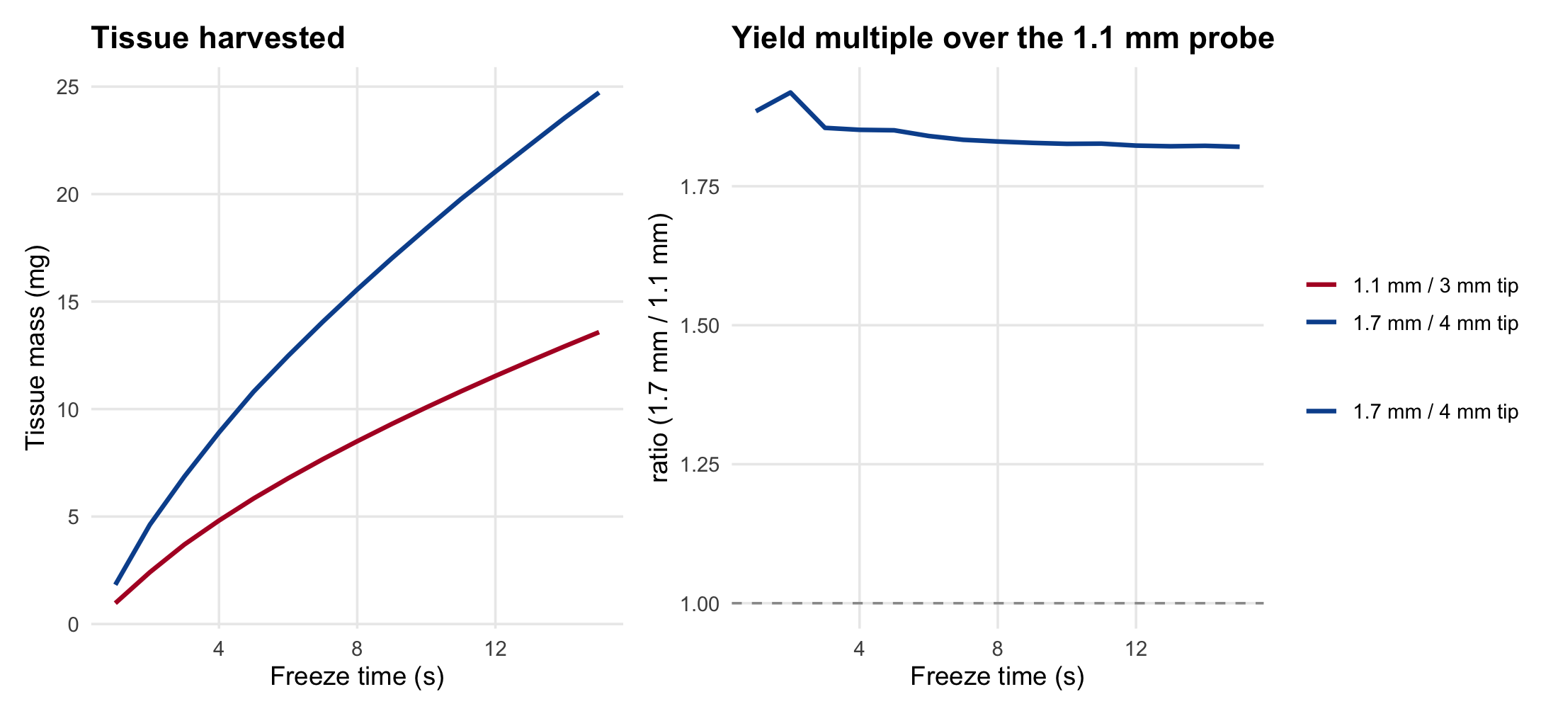
Where the extra tissue comes from
res |> filter(t %in% c(5, 10)) |>
  select(probe, t, D_max, wall_ice, L_axial, V_ice) |>
  pivot_wider(names_from = t, values_from = c(D_max, wall_ice, L_axial, V_ice)) |>
  transmute(Probe = probe,
            `Collar 5s (mm)` = round(wall_ice_5, 2),
            `Collar 10s (mm)` = round(wall_ice_10, 2),
            `Diameter 5s (mm)` = round(D_max_5, 2),
            `Length 5s (mm)` = round(L_axial_5, 2),
            `Volume 5s (mm3)` = round(V_ice_5, 1),
            `Volume 10s (mm3)` = round(V_ice_10, 1)) |>
  kable(caption = paste("Frozen collar thickness is the radial distance from the probe",
"wall to the 0 C front."))| Probe | Collar 5s (mm) | Collar 10s (mm) | Diameter 5s (mm) | Length 5s (mm) | Volume 5s (mm3) | Volume 10s (mm3) |
|---|---|---|---|---|---|---|
| 1.1 mm / 3 mm tip | 1.04 | 1.43 | 3.19 | 4.51 | 24.2 | 41.8 |
| 1.7 mm / 4 mm tip | 1.10 | 1.53 | 3.91 | 5.70 | 44.8 | 76.4 |
The collar thickness on the 1.1 mm probe at 10 s is 1.43 mm against 1.53 mm on the 1.7 mm probe. The two are close, which is the essential point: both probes grow a collar of similar thickness, so the extra yield of the larger probe comes almost entirely from wrapping that collar around a bigger cylinder, not from freezing any faster.
Diameter or tip length? (hypothetical decomposition)
The 1.7 mm probe is both wider and longer-tipped than the 1.1 mm probe, so its advantage mixes two causes. To separate them we simulate a hypothetical 1.7 mm probe with a 3 mm tip - matching the small probe’s tip length - so that diameter is the only difference. This device does not exist; it is a decomposition aid only.
s_h <- run_cryo(modifyList(P0, hypo_cfg))
hyp <- bind_rows(lapply(s_h$snaps, ice_metrics, g = s_h$grid, P = s_h$P))

dec <- res |> filter(t %in% c(5, 10)) |> select(probe, t, tissue_mg) |>
  bind_rows(hyp |> filter(t %in% c(5,10)) |>
              transmute(probe = "1.7 mm / 3 mm tip (hypothetical)", t, tissue_mg))
sm <- dec |> filter(probe == "1.1 mm / 3 mm tip") |> select(t, small = tissue_mg)

dec |> filter(probe != "1.1 mm / 3 mm tip") |> left_join(sm, by = "t") |>
  mutate(ratio = tissue_mg/small) |>
  select(probe, t, ratio) |>
  pivot_wider(names_from = t, values_from = ratio, names_prefix = "t") |>
  transmute(`Compared with the 1.1 mm probe` = probe,
            `ratio at 5 s` = round(t5, 2), `ratio at 10 s` = round(t10, 2)) |>
kable(caption = "Splitting the 1.7 mm advantage into diameter and tip length.")| Compared with the 1.1 mm probe | ratio at 5 s | ratio at 10 s |
|---|---|---|
| 1.7 mm / 4 mm tip | 1.85 | 1.83 |
| 1.7 mm / 3 mm tip (hypothetical) | 1.44 | 1.43 |
Of the total 1.85x advantage at 5 s, diameter alone accounts for 1.44x and the extra millimetre of tip supplies the remaining 1.28x. The diameter term sits just below the 1.55 ratio of the probe radii, which is what one would expect if the frozen collar simply wrapped a larger cylinder.
Shapes, drawn to the same scale
fr <- bind_rows(lapply(names(sims), function(nm) {
  s <- sims[[nm]]
  bind_rows(lapply(s$snaps[sapply(s$snaps, `[[`, "t") %in% c(5, 10)],
                   front_df, g = s$grid, P = s$P, lab = nm))
})) |> mutate(tlab = factor(paste0(t, " s"), levels = c("5 s","10 s")),
              lab = factor(lab, levels = names(probe_cfg)))

rects <- bind_rows(lapply(names(probe_cfg), function(nm) {
  cf <- probe_cfg[[nm]]; L <- cf$Ltip*1e3; a <- cf$a*1e3
  data.frame(lab = nm, what = c("shaft","tip"),
             xmin = c(-L-4, -L), xmax = c(-L, 0), ymin = -a, ymax = a)
})) |> mutate(lab = factor(lab, levels = names(probe_cfg)))

ggplot(fr, aes(x, y, group = interaction(grp, lab))) +
  geom_polygon(fill = "#9EC9EC", colour = "#12508F", linewidth = 0.55) +
  geom_rect(data = filter(rects, what == "shaft"), inherit.aes = FALSE,
            aes(xmin=xmin, xmax=xmax, ymin=ymin, ymax=ymax),
            fill = "grey70", colour = "grey40", linewidth = 0.3) +
  geom_rect(data = filter(rects, what == "tip"), inherit.aes = FALSE,
            aes(xmin=xmin, xmax=xmax, ymin=ymin, ymax=ymax),
            fill = "grey25", colour = "grey15", linewidth = 0.3) +
  facet_grid(tlab ~ lab) +
  coord_fixed(xlim = c(-9.5, 3.5), ylim = c(-3.4, 3.4)) +
  labs(title = "Frozen specimen by probe, aligned at the distal tip apex",
       subtitle = "Same scale throughout; grey = probe, blue = frozen lung",
       x = "Axial distance from distal tip apex (mm)", y = "Radius (mm)")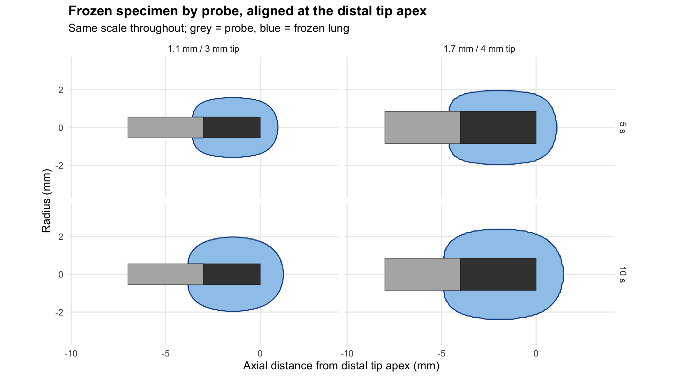
How much longer must the 1.1 mm probe freeze to catch up?
A fair way to state the penalty is as a time cost: for a given 1.7 mm freeze, how long must the 1.1 mm probe be held to harvest the same mass of tissue?
small <- res |> filter(probe == "1.1 mm / 3 mm tip") |> arrange(t)
match_t <- function(target_mg) {
  if (target_mg > max(small$tissue_mg)) return(NA_real_)
  approx(small$tissue_mg, small$t, target_mg)$y
}
equiv <- res |> filter(probe != "1.1 mm / 3 mm tip", t %in% c(3, 5, 7, 10)) |>
  rowwise() |>
  mutate(t_equiv = match_t(tissue_mg)) |>
  ungroup()

equiv |> transmute(`1.7 mm configuration` = probe,
                   `1.7 mm freeze (s)` = t,
                   `Tissue mass (mg)` = round(tissue_mg, 2),
                   `1.1 mm freeze needed (s)` = round(t_equiv, 1),
                   `Extra seconds` = round(t_equiv - t, 1)) |>
  kable(caption = paste("Freeze time the 1.1 mm probe needs to match the 1.7 mm probe.",
"NA = unreachable within 15 s."))| 1.7 mm configuration | 1.7 mm freeze (s) | Tissue mass (mg) | 1.1 mm freeze needed (s) | Extra seconds |
|---|---|---|---|---|
| 1.7 mm / 4 mm tip | 3 | 6.86 | 6.1 | 3.1 |
| 1.7 mm / 4 mm tip | 5 | 10.80 | 11.0 | 6.0 |
| 1.7 mm / 4 mm tip | 7 | 14.05 | NA | NA |
| 1.7 mm / 4 mm tip | 10 | 18.40 | NA | NA |
ggplot(res, aes(t, tissue_mg, colour = probe)) +
  geom_line(linewidth = 1) +
  geom_segment(data = filter(equiv, !is.na(t_equiv)),
               aes(x = t, xend = t_equiv, y = tissue_mg, yend = tissue_mg),
               linetype = "dotted", colour = "grey40", inherit.aes = FALSE) +
  geom_point(data = filter(equiv, !is.na(t_equiv)),
             aes(x = t_equiv, y = tissue_mg), colour = "#B2182B", size = 1.8,
             inherit.aes = FALSE) +
  scale_colour_manual(values = PROBE_COLS, name = NULL) +

  labs(title = "Matching the 1.7 mm probe's yield with the 1.1 mm probe",
       subtitle = "Dotted lines show the extra freeze time required",
       x = "Freeze time (s)", y = "Tissue mass (mg)")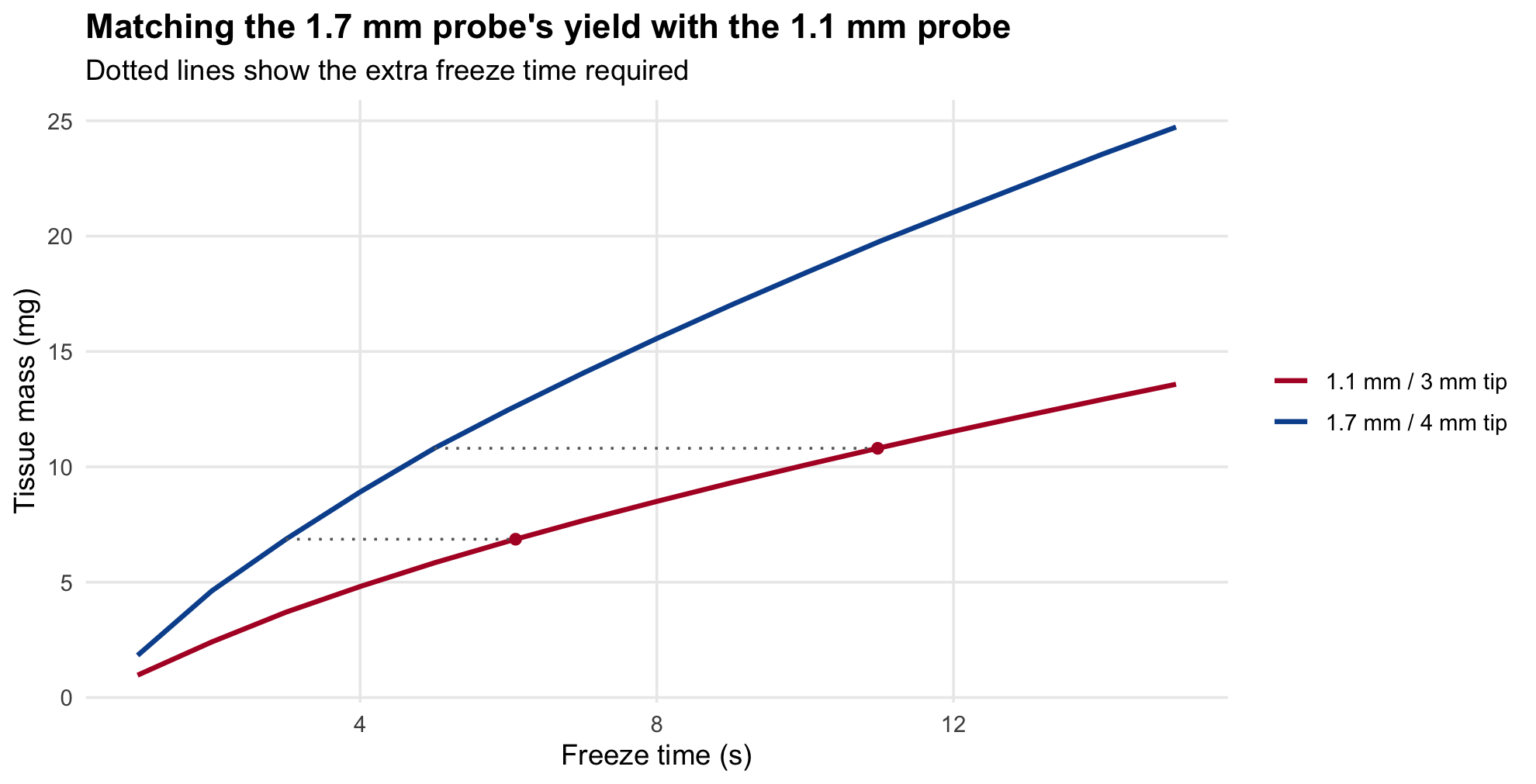
Does the conclusion hold across aeration?
The previous study found the frozen volume to be almost independent of tissue fraction while the harvested mass scales with it. If both probes respond the same way, the ratio between them should be robust. That is worth checking rather than assuming.
ft_grid <- c(0.10, 0.142, 0.241, 0.40, 0.60)
sweep <- bind_rows(lapply(ft_grid, function(f)
  bind_rows(lapply(names(probe_cfg), function(nm) {
    cf <- probe_cfg[[nm]]
    Pi <- modifyList(modifyList(P0, cf), list(ft = f, dx = cf$dx * 2))
    s <- run_cryo(Pi, snap_times = c(5, 10, 15), n_rec = 6)
    bind_rows(lapply(s$snaps, ice_metrics, g = s$grid, P = Pi)) |>
      mutate(probe = nm, ft = f)
  }))))
sw_small <- sweep |> filter(probe == "1.1 mm / 3 mm tip") |>
select(ft, t, small = tissue_mg)
sw_r <- sweep |> filter(probe != "1.1 mm / 3 mm tip") |>
left_join(sw_small, by = c("ft","t")) |> mutate(ratio = tissue_mg/small)
sw_r |> select(probe, ft, t, ratio) |>
pivot_wider(names_from = t, values_from = ratio, names_prefix = "t") |>
transmute(`1.7 mm configuration` = probe, `f_t` = ft,
`ratio 5 s` = round(t5, 2), `ratio 10 s` = round(t10, 2),
`ratio 15 s` = round(t15, 2)) |>
kable(caption = "Yield multiple across aeration (coarse grid). Stable = conclusion is robust.")| 1.7 mm configuration | f_t | ratio 5 s | ratio 10 s | ratio 15 s |
|---|---|---|---|---|
| 1.7 mm / 4 mm tip | 0.100 | 1.80 | 1.81 | 1.80 |
| 1.7 mm / 4 mm tip | 0.142 | 1.79 | 1.80 | 1.79 |
| 1.7 mm / 4 mm tip | 0.241 | 1.78 | 1.79 | 1.77 |
| 1.7 mm / 4 mm tip | 0.400 | 1.77 | 1.77 | 1.77 |
| 1.7 mm / 4 mm tip | 0.600 | 1.76 | 1.76 | 1.76 |
Numerical verification of the ratio
Absolute volumes carry a few percent of discretisation error. The ratio between two probes is the quantity being reported, so it is the ratio whose convergence matters. Note that because each probe is run at its own cell size, the two errors do not cancel the way they would on a shared grid - so this check is a genuine test, not a formality.
## halving the resolution of BOTH probes and re-forming the ratio
conv <- bind_rows(lapply(c(1, 2), function(mult)
  bind_rows(lapply(names(probe_cfg), function(nm) {
    cf <- probe_cfg[[nm]]
    Pi <- modifyList(modifyList(P0, cf), list(dx = cf$dx * mult))
    s <- run_cryo(Pi, snap_times = c(5, 10, 15), n_rec = 6)
    bind_rows(lapply(s$snaps, ice_metrics, g = s$grid, P = Pi)) |>
      mutate(probe = nm, grid = ifelse(mult == 1, "fine", "coarse"))
  }))))

cs <- conv |> filter(probe == "1.1 mm / 3 mm tip") |> select(grid, t, small = tissue_mg)
conv |> filter(probe != "1.1 mm / 3 mm tip") |>
  left_join(cs, by = c("grid","t")) |>
  mutate(ratio = tissue_mg/small) |>
  select(probe, grid, t, ratio) |>
  pivot_wider(names_from = grid, values_from = ratio) |>
  transmute(`1.7 mm configuration` = probe, `t (s)` = t,
            `ratio, coarse` = round(coarse, 2), `ratio, fine` = round(fine, 2),
            `change %` = round(100*(fine-coarse)/fine, 1)) |>
  kable(caption = paste("Grid sensitivity of the yield ratio. The two probes are run",
                        "at different cell sizes, so their discretisation errors do not",
"fully cancel; the ratio carries about 3% numerical uncertainty."))| 1.7 mm configuration | t (s) | ratio, coarse | ratio, fine | change % |
|---|---|---|---|---|
| 1.7 mm / 4 mm tip | 5 | 1.78 | 1.85 | 3.8 |
| 1.7 mm / 4 mm tip | 10 | 1.79 | 1.83 | 2.2 |
| 1.7 mm / 4 mm tip | 15 | 1.77 | 1.82 | 2.6 |
Interpretation
The answer
At a clinically typical 5 s freeze, the 1.7 mm probe with its 4 mm tip returns 1.85x the tissue of the 1.1 mm probe with its 3 mm tip. The multiple is strikingly stable with freeze time - 1.86x at 3 s and 1.82x at 15 s - so it can be carried around as a single number rather than a curve.
Equivalently, the 1.1 mm probe harvests about 54% of the tissue the 1.7 mm probe does at the same freeze time.
The decomposition above attributes roughly 1.44x of that to the larger diameter and the remaining 1.28x to the longer tip.
The time cost, and why it does not close the gap
The 1.1 mm probe cannot simply be frozen longer to compensate. Because growth decelerates so steeply, matching even a 5 s freeze of the 1.7 mm / 4 mm probe requires 11 s, and matching a 7 s freeze requires more than 15 s - it is unreachable. Freeze time is a poor substitute for probe diameter. Doubling the freeze buys well under double the tissue, whereas the diameter penalty applies from the first second.
What this does and does not imply clinically
This is a thermal model, and yield is only one axis of the decision. Three caveats matter before drawing a clinical conclusion:
- A larger frozen mass is also a larger tear. The 1.7 mm probe’s advantage in tissue is accompanied by a proportionally larger ice ball being avulsed, which is the mechanical origin of bleeding and pneumothorax risk. This model quantifies the benefit, not the harm, and the two scale together.
- The 1.1 mm probe reaches places the 1.7 mm cannot. Nothing here models trafficability, working-channel compatibility, or how peripherally each probe can be navigated. A smaller specimen from the correct location beats a larger one from the wrong one.
- Adequacy is a threshold, not a linear scale. Diagnostic yield in DPLD depends on whether the specimen contains enough alveolated parenchyma to show a pattern. A 1.9x mass advantage does not translate into a 1.9x diagnostic advantage, and the published comparison of 1.7 mm against 1.9 mm probes found similar diagnostic yield despite a similar size difference - consistent with both being above the adequacy threshold.
The defensible summary is therefore narrow and physical: the 1.1 mm probe harvests roughly 0.54 of the tissue mass of a 1.7 mm probe with a 4 mm tip at equal freeze time, and cannot close that gap by freezing longer. Whether that matters diagnostically is an empirical question this model cannot answer.
Limitations
All limitations of the previous study carry over unchanged: continuum homogenisation below the alveolar scale, a prescribed rather than solved tip temperature, no contact resistance, and the ice ball being an upper bound on what actually detaches.
The mixing-model uncertainty - which dominated the previous study - also carries over, but it should largely cancel in a ratio taken within the same medium. Rather than assert that, we test it:
mix_r <- bind_rows(lapply(c("emt","me","par"), function(mm)
  bind_rows(lapply(names(probe_cfg), function(nm) {
    cf <- probe_cfg[[nm]]
    Pi <- modifyList(modifyList(P0, cf), list(mix = mm, dx = cf$dx*2))
    s <- run_cryo(Pi, snap_times = c(5, 10), n_rec = 5)
    bind_rows(lapply(s$snaps, ice_metrics, g = s$grid, P = Pi)) |>
      mutate(probe = nm, model = mm)
  }))))

mr_small <- mix_r |> filter(probe == "1.1 mm / 3 mm tip") |>
  select(model, t, small = tissue_mg)
mix_r |> filter(probe != "1.1 mm / 3 mm tip") |>
  left_join(mr_small, by = c("model","t")) |>
  mutate(ratio = tissue_mg/small) |>
  select(probe, model, t, ratio) |>
  pivot_wider(names_from = t, values_from = ratio, names_prefix = "t") |>
  transmute(`1.7 mm configuration` = probe,
            `Mixing model` = recode(model, emt = "Bruggeman EMT",
                                    me = "Maxwell-Eucken", par = "Parallel"),
            `ratio 5 s` = round(t5, 2), `ratio 10 s` = round(t10, 2)) |>
  arrange(`1.7 mm configuration`) |>
kable(caption = "Yield ratio under each conductivity mixing model.")| 1.7 mm configuration | Mixing model | ratio 5 s | ratio 10 s |
|---|---|---|---|
| 1.7 mm / 4 mm tip | Bruggeman EMT | 2.01 | 1.91 |
| 1.7 mm / 4 mm tip | Maxwell-Eucken | 1.78 | 1.79 |
| 1.7 mm / 4 mm tip | Parallel | 1.78 | 1.77 |
The ratio moves only between 1.77 and 2.01 across the three models - a spread of about 13% - where the absolute diameters those same models predict differ by nearly a factor of two. Cancellation is not perfect: Bruggeman EMT, with its far lower conductivity, slightly favours the larger probe. But this is why the yield multiple is considerably more trustworthy than any absolute volume in these documents - the dominant modelling uncertainty acts on both probes alike and largely divides out. The comparison is on firmer ground than either study’s standalone predictions.