
MLE and the optimal classification threshold
Contents
The argument
A datamethods thread caught my attention because it deals with the classification problem so common in medicine and its downstream elements (ROC AUC, thresholds etc). It started with the observation that the Youden index, the conventional way to pick a cutoff, is built from sensitivity and specificity, which describe classifying outcomes one already knows. For predicting unknown outcomes the poster proposed a “P-index” — the threshold maximizing PPV + NPV — and argued that AUROC is the wrong performance measure.
Frank Harrell disagreed, on grounds worth repeating exactly:
Maximum likelihood estimation (or the Bayesian extension of it) is what gives us optimum prediction.
and
It is a mistake to consider thresholds when building a model.
He separates models from decisions and states that thresholds belong to decisions, not to models. A threshold requires a utility function, and that utility may differ from patient to patient. If you must dichotomise, you dichotomise the model’s output — never the covariates — in a way that approximates maximising expected utility. Aother poster supplied the theoretical backing, Gneiting & Raftery (2007) on strictly proper scoring rules: a scoring rule is proper when reporting your true probability maximises your expected score, and maximum likelihood uses the logarithmic rule, which is strictly proper.
This post works through the mechanics in R. We fit by maximum
likelihood, twice — once by hand so the likelihood is not a black box,
then with one my favorite R packages, rms — and only
afterwards ask where a cutoff could come from. Then we compute the
Youden index and show, numerically, exactly what assumption it is making
on your behalf.
A toy dataset
A simulated diagnostic problem, so we know the truth. Risk depends on age, a standardised biomarker, and sex.
set.seed(2026)
n <- 1000

age <- round(rnorm(n, 62, 10))
bm  <- rnorm(n)
sex <- factor(sample(c("F", "M"), n, replace = TRUE))

lp <- -1.8 + 0.045 * (age - 62) + 1.15 * bm + 0.35 * (sex == "M")
d  <- data.frame(y = rbinom(n, 1, plogis(lp)), age, bm, sex)
head(d)
## y age bm sex
## 1 1 67 1.7705647 F
## 2 1 51 0.9003771 M
## 3 0 63 1.3304134 M
## 4 0 61 -0.3492971 M
## 5 1 55 1.0621850 F
## 6 0 37 -0.6199544 Fprev <- mean(d$y)
prev## [1] 0.188The true coefficients are (-1.8, 0.045, 1.15, 0.35) and
the prevalence is about 19%. Keep both in mind — the prevalence returns
in section 7 in a way that is not a coincidence.
What maximum likelihood actually is
For a binary outcome with \(P(y_i = 1) = p_i\) and \(\text{logit}(p_i) = x_i'\beta\), the log-likelihood is
\[\ell(\beta) = \sum_i \left[ y_i \, x_i'\beta - \log\left(1 + e^{x_i'\beta}\right) \right]\]
Nothing here mentions a threshold. The estimate is the \(\beta\) making the observed data most probable, and because the logarithmic scoring rule is strictly proper, the fitted probabilities are the ones you should report.
Coding it directly is worth doing once. Note
log1p(exp(eta)) rather than log(1 + exp(eta))
— it is the numerically stable form:
X <- model.matrix(~ age + bm + sex, data = d)

neg_loglik <- function(beta) {
  eta <- as.vector(X %*% beta)
  -sum(d$y * eta - log1p(exp(eta)))
}

# the score function: the gradient of the log-likelihood is X'(y - p).
# Supplying it analytically is not optional here - with a purely numerical
# gradient BFGS stops well short of the optimum, off in the second decimal.
neg_score <- function(beta) {
  p <- plogis(as.vector(X %*% beta))
  -as.vector(t(X) %*% (d$y - p))
}

fit_optim <- optim(rep(0, ncol(X)),
                   neg_loglik,
                   gr = neg_score, method = "BFGS", hessian = TRUE,
                   control = list(reltol = 1e-14, maxit = 1000))

# the inverse Hessian of the NEGATIVE log-likelihood is the covariance matrix
se_optim <- sqrt(diag(solve(fit_optim$hessian)))

round(cbind(estimate = fit_optim$par, SE = se_optim), 4)
## estimate SE
## [1,] -5.1240 0.6372
## [2,] 0.0490 0.0095
## [3,] 1.1673 0.1094
## [4,] 0.4758 0.1810That is maximum likelihood with no package at all: a log-likelihood, an optimiser, and the second derivative for standard errors.
The same fit in rms
lrm() does the same thing with better numerics and a
great deal more machinery attached.
dd <- datadist(d)

# rms stores only the NAME of the datadist object and looks it up in the global
# environment. knitr evaluates each chunk in its own environment, so inside an
# .Rmd this assignment is required - without it lrm() fails with
# "dataset dd not found for options(datadist=)".
assign("dd", dd, envir = globalenv())
options(datadist = "dd")

f <- lrm(y ~ age + bm + sex, data = d, x = TRUE, y = TRUE)
f
## Logistic Regression Model
##
## lrm(formula = y ~ age + bm + sex, data = d, x = TRUE, y = TRUE)
##
## Model Likelihood Discrimination Rank Discrim.
## Ratio Test Indexes Indexes
## Obs 1000 LR chi2 172.10 R2 0.255 C 0.781
## 0 812 d.f. 3 R2(3,1000)0.156 Dxy 0.563
## 1 188 Pr(> chi2) <0.0001 R2(3,458)0.309 gamma 0.563
## max |deriv| 1e-08 Brier 0.124 tau-a 0.172
##
## Coef S.E. Wald Z Pr(>|Z|)
## Intercept -5.1240 0.6369 -8.05 <0.0001
## age 0.0490 0.0095 5.17 <0.0001
## bm 1.1673 0.1094 10.67 <0.0001
## sex=M 0.4758 0.1810 2.63 0.0086The two agree to optimiser tolerance:
round(max(abs(coef(f) - fit_optim$par)), 6)## [1] 0lrm prints what Harrell recommends in place of
threshold-based summaries: the likelihood-ratio \(\chi^2\), Nagelkerke’s \(R^2\), Somers’ \(D_{xy}\), the \(c\)-index, and the Brier score — all
computed from probabilities, none requiring a cutoff. Validate them with
the bootstrap to see the optimism:
set.seed(11)
validate(f, B = 200)
## index.orig training test optimism index.corrected Lower Upper
## Dxy 0.5629 0.5666 0.5598 0.0069 0.5560 0.4795 0.6297
## R2 0.2552 0.2606 0.2524 0.0082 0.2470 0.1763 0.3108
## Intercept 0.0000 0.0000 -0.0218 0.0218 -0.0218 -0.3183 0.3382
## Slope 1.0000 1.0000 0.9811 0.0189 0.9811 0.7730 1.2125
## Emax 0.0000 0.0000 0.0375 -0.0375 0.0375 -0.0069 0.1160
## D 0.1711 0.1755 0.1691 0.0064 0.1647 0.1099 0.2131
## U -0.0020 -0.0020 0.0001 -0.0021 0.0001 -0.0032 0.0088
## Q 0.1731 0.1775 0.1690 0.0084 0.1647 0.1044 0.2133
## B 0.1238 0.1230 0.1244 -0.0014 0.1251 0.1135 0.1398
## g 1.3922 1.4180 1.3813 0.0367 1.3555 1.0626 1.5985
## gp 0.1741 0.1755 0.1731 0.0024 0.1717 0.1429 0.1981
## n
## Dxy 200
## R2 200
## Intercept 200
## Slope 200
## Emax 200
## D 200
## U 200
## Q 200
## B 200
## g 200
## gp 200The index.corrected column is the honest estimate.
Calibration matters at least as much as discrimination, because a
threshold applied to a miscalibrated probability is meaningless:
set.seed(12)
cal <- calibrate(f, B = 200)

cal_df <- data.frame(
  predicted = as.numeric(cal[, "predy"]),
  apparent  = as.numeric(cal[, "calibrated.orig"]),
  corrected = as.numeric(cal[, "calibrated.corrected"])
)

ggplot(cal_df, aes(x = predicted)) +
  geom_abline(slope = 1, intercept = 0, linetype = "dashed", colour = "grey40") +
  geom_line(aes(y = apparent,  colour = "Apparent"),  linewidth = 0.9) +
  geom_line(aes(y = corrected, colour = "Bias-corrected"), linewidth = 0.9) +
  scale_colour_manual(values = c("Apparent" = "#268bd2",
                                 "Bias-corrected" = "#d33682"),
                      name = NULL) +
  coord_fixed() +
  labs(title = "Calibration of the MLE fit",
       subtitle = "Dashed line is perfect calibration; 200 bootstrap resamples",
       x = "Predicted probability", y = "Observed proportion")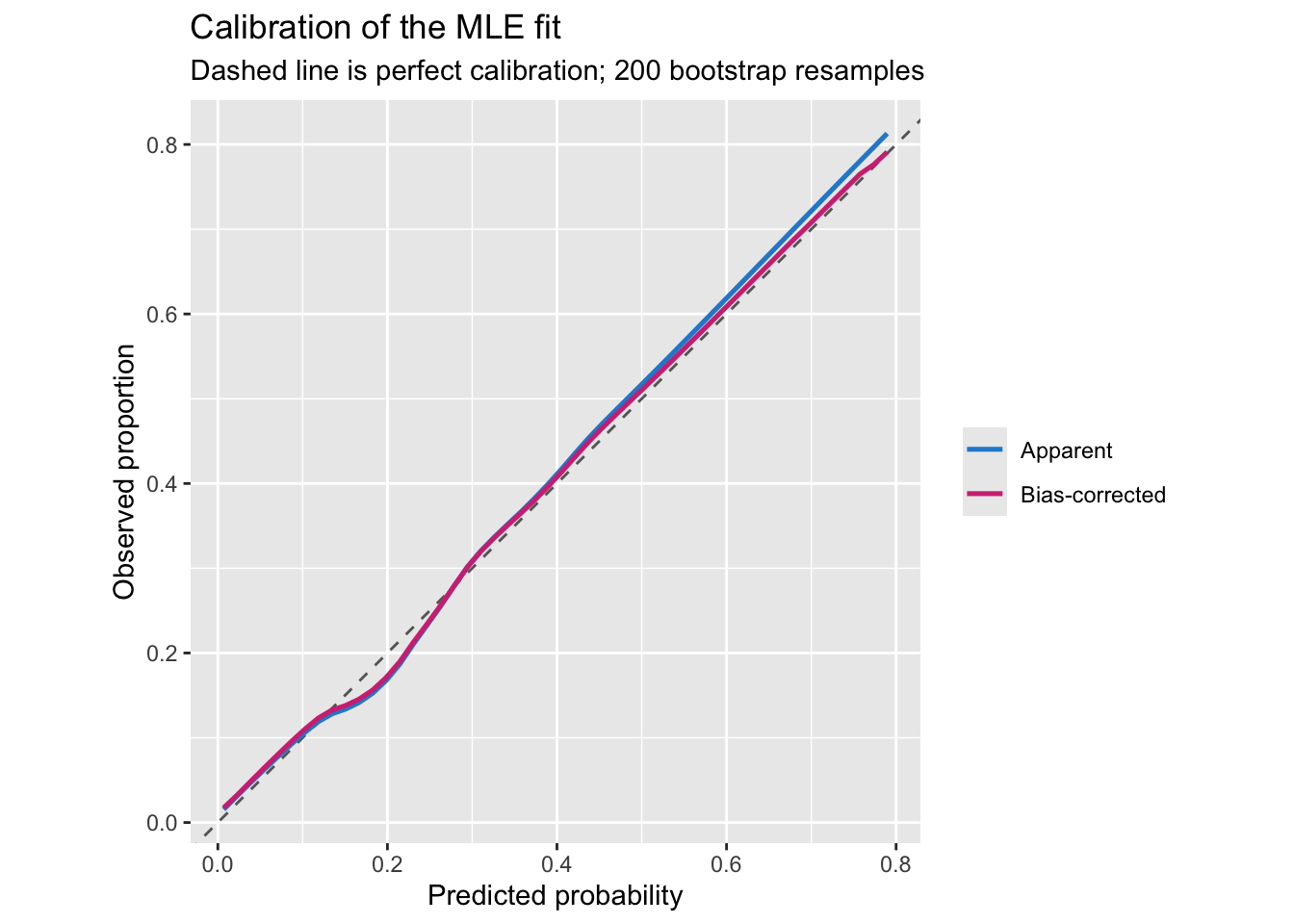
Where a threshold comes from
Only now does a cutoff become a sensible question — and it is answered by costs, not by data. Consider one patient with estimated risk \(p\). Let \(C_{FP}\) be the cost of treating someone who did not need it and \(C_{FN}\) the cost of failing to treat someone who did. Expected losses:
\[\text{treat} : (1 - p)\,C_{FP} \qquad\qquad \text{don't treat} : p\,C_{FN}\]
Treat when the first is smaller, which rearranges to
\[p > p^* = \frac{C_{FP}}{C_{FP} + C_{FN}}\]
The threshold is a statement about values, and the data never enter it. Equal costs give \(p^* = 0.5\); a false negative nine times worse than a false positive gives \(p^* = 0.1\).
p_star <- function(C_FP, C_FN) C_FP / (C_FP + C_FN)

data.frame(C_FP = c(1, 1, 1, 2),
           C_FN = c(1, 3, 9, 1),
           p_star = p_star(c(1, 1, 1, 2), c(1, 3, 9, 1)))
## C_FP C_FN p_star
## 1 1 1 0.5000000
## 2 1 3 0.2500000
## 3 1 9 0.1000000
## 4 2 1 0.6666667We can check this against the empirical loss on our own data:
ph <- predict(f, type = "fitted")

expected_loss <- function(t, C_FP, C_FN)
  (C_FP * sum(ph >= t & d$y == 0) + C_FN * sum(ph < t & d$y == 1)) / length(d$y)

grid <- seq(0.005, 0.995, by = 0.005)
loss_df <- data.frame(t = grid, loss = sapply(grid, expected_loss, 1, 9))

c(theory = p_star(1, 9), empirical = grid[which.min(loss_df$loss)])
## theory empirical
## 0.100 0.095ggplot(loss_df, aes(t, loss)) +
geom_line(linewidth = 0.9, colour = "#268bd2") +
geom_vline(xintercept = p_star(1, 9), linetype = "dashed", colour = "#d33682") +
annotate("text", x = p_star(1, 9), y = max(loss_df$loss), hjust = -0.1,
label = "p* = 0.1 from costs", colour = "#d33682", size = 3.4) +
labs(title = "Expected loss when a false negative costs nine false positives",
subtitle = "The cost-derived threshold sits at the minimum",
x = "Threshold", y = "Expected loss per patient")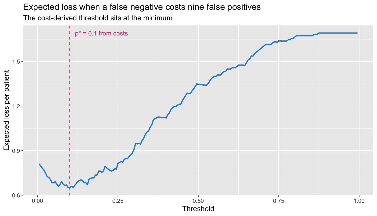
The Youden index
Youden’s \(J\) maximises \(\text{sensitivity} + \text{specificity} - 1\). It uses no costs at all, which is exactly the problem — but first, the computation.
roc_points <- function(ph, y) {
  g <- sort(unique(ph))
  data.frame(
    t    = g,
    sens = sapply(g, function(t) mean(ph[y == 1] >= t)),
    spec = sapply(g, function(t) mean(ph[y == 0] <  t))
  )
}

roc <- roc_points(ph, d$y)
roc$J <- roc$sens + roc$spec - 1

t_youden <- roc$t[which.max(roc$J)]
c(threshold = t_youden, J = max(roc$J))
## threshold J
## 0.2469730 0.4457866The \(c\)-index from
lrm is the area under this same curve, and
Hmisc::somers2 confirms it:
c(lrm = unname(f$stats["C"]), somers2 = unname(somers2(ph, d$y)["C"]))## lrm somers2
## 0.7814563 0.7814563pt <- function(th) {
i <- which.min(abs(roc$t - th))
data.frame(fpr = 1 - roc$spec[i], sens = roc$sens[i])
}
marks <- rbind(
cbind(pt(t_youden), rule = "Youden (J max)"),
cbind(pt(p_star(1, 9)), rule = "Cost-derived (p* = 0.1)")
)
ggplot(roc, aes(1 - spec, sens)) +
geom_abline(slope = 1, intercept = 0, linetype = "dashed", colour = "grey60") +
geom_line(linewidth = 0.9, colour = "#268bd2") +
geom_point(data = marks, aes(fpr, sens, colour = rule), size = 3) +
scale_colour_manual(values = c("Youden (J max)" = "#d33682",
"Cost-derived (p* = 0.1)" = "#859900"),
name = NULL) +
coord_fixed() +
labs(title = "Two operating points on one ROC curve",
subtitle = "Same model, same data, different questions",
x = "1 - specificity", y = "Sensitivity")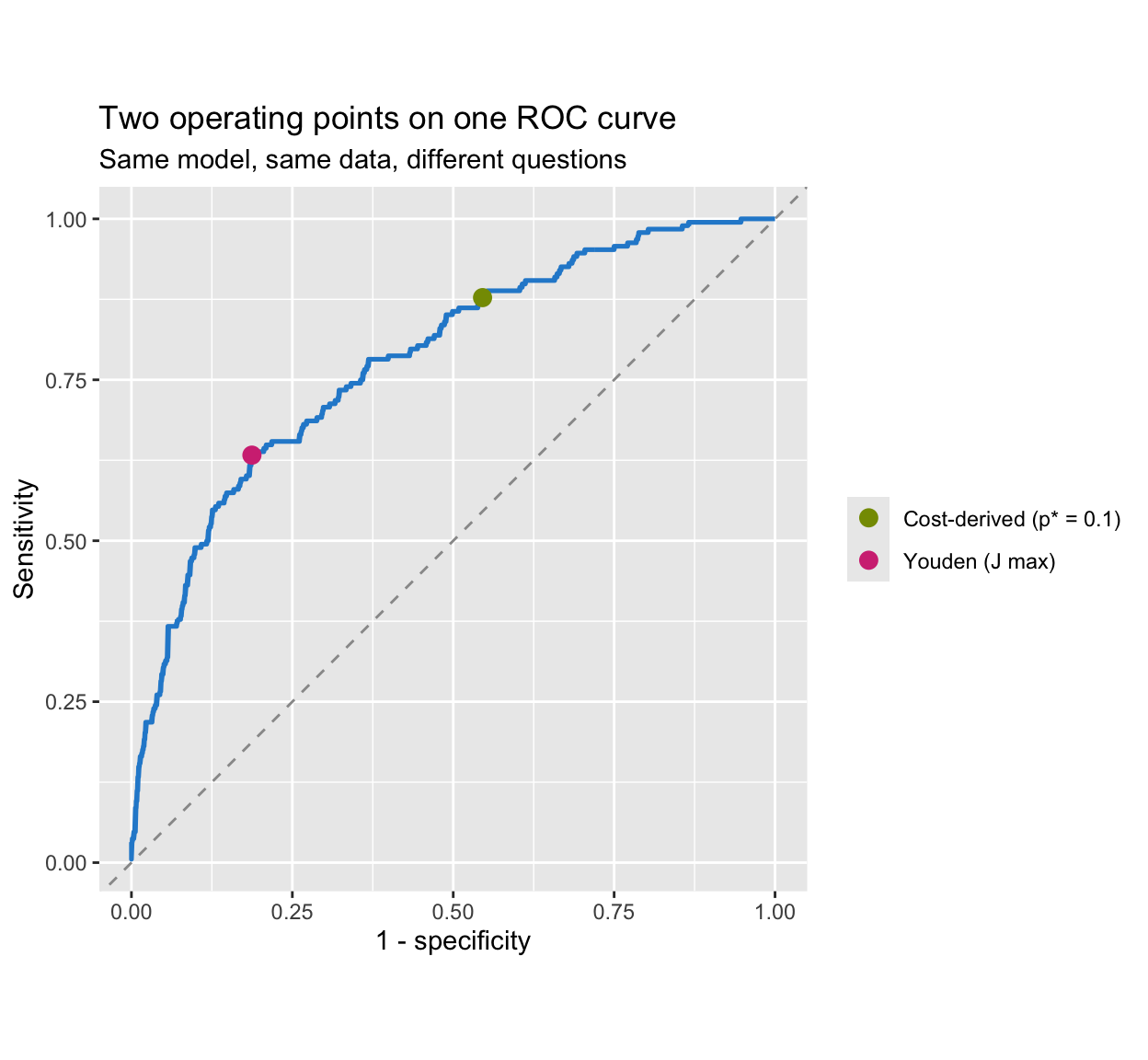
They are different points. Only one of them answers a question anybody asked.
What Youden silently assumes
Youden is not cost-free; it is cost-implicit. The optimal operating point on an ROC curve is where the tangent has slope
\[\frac{1 - \pi}{\pi} \cdot \frac{C_{FP}}{C_{FN}}\]
with \(\pi\) the prevalence. Maximising \(\text{sens} + \text{spec} - 1\) is maximising vertical distance above the diagonal, which happens where the slope equals 1. Setting the two equal:
\[\frac{C_{FP}}{C_{FN}} = \frac{\pi}{1 - \pi} \qquad\Longrightarrow\qquad p^* = \frac{C_{FP}}{C_{FP} + C_{FN}} = \pi\]
Youden’s threshold is the prevalence. Not approximately, as a large-sample matter — it is what maximising \(J\) means. Our data:
c(youden_threshold = t_youden,
  prevalence       = prev,
  implied_C_FN_over_C_FP = (1 - prev) / prev)
## youden_threshold prevalence implied_C_FN_over_C_FP
## 0.246973 0.188000 4.319149With 19% prevalence, choosing Youden asserts that a missed case is about 4.3 times as costly as a false alarm. That may be true. The point is that nobody decided it — the prevalence did. Change the case mix and your implied values change with it, which is not how values work.
At \(n = 1000\) the match is rough. It tightens as the curve smooths out:
sim_once <- function(n, seed) {
  set.seed(seed)
  a <- round(rnorm(n, 62, 10)); b <- rnorm(n)
  s <- factor(sample(c("F", "M"), n, replace = TRUE))
  dat <- data.frame(y = rbinom(n, 1, plogis(-1.8 + 0.045*(a-62) + 1.15*b + 0.35*(s=="M"))),
                    age = a, bm = b, sex = s)
  p <- fitted(glm(y ~ age + bm + sex, data = dat, family = binomial))
  r <- roc_points(p, dat$y)
  c(prevalence = mean(dat$y), youden = r$t[which.max(r$sens + r$spec - 1)])
}

do.call(rbind, lapply(c(500, 2000, 20000), function(n) {
  out <- t(sapply(1:5, function(s) sim_once(n, 100 + s)))
  data.frame(n = n,
             prevalence = round(mean(out[, "prevalence"]), 3),
             youden_mean = round(mean(out[, "youden"]), 3),
             youden_sd   = round(sd(out[, "youden"]), 3))
}))
## n prevalence youden_mean youden_sd
## 1 500 0.227 0.229 0.048
## 2 2000 0.220 0.224 0.033
## 3 20000 0.221 0.222 0.010The two columns converge. The last column is the subject of the next section.
The cutoff is unstable
Even granting Youden’s implied costs, the cutoff is estimated badly. Bootstrap it:
set.seed(99)
boot_youden <- replicate(500, {
  i  <- sample(nrow(d), replace = TRUE)
  fb <- glm(y ~ age + bm + sex, data = d[i, ], family = binomial)
  pb <- fitted(fb)
  rb <- roc_points(pb, d$y[i])
  rb$t[which.max(rb$sens + rb$spec - 1)]
})

round(quantile(boot_youden, c(0.025, 0.25, 0.5, 0.75, 0.975)), 3)
## 2.5% 25% 50% 75% 97.5%
## 0.151 0.210 0.242 0.268 0.307ggplot(data.frame(t = boot_youden), aes(t)) +
geom_histogram(bins = 40, fill = "#268bd2", colour = "white") +
geom_vline(xintercept = t_youden, colour = "#d33682", linewidth = 0.9) +
geom_vline(xintercept = p_star(1, 9), colour = "#859900",
linewidth = 0.9, linetype = "dashed") +
labs(title = "500 bootstrap replicates of the Youden cutoff",
subtitle = paste("Magenta: the cutoff from the observed data.",
"Green dashed: a cost-derived threshold, which does not vary at all."),
x = "Youden-optimal threshold", y = "Count")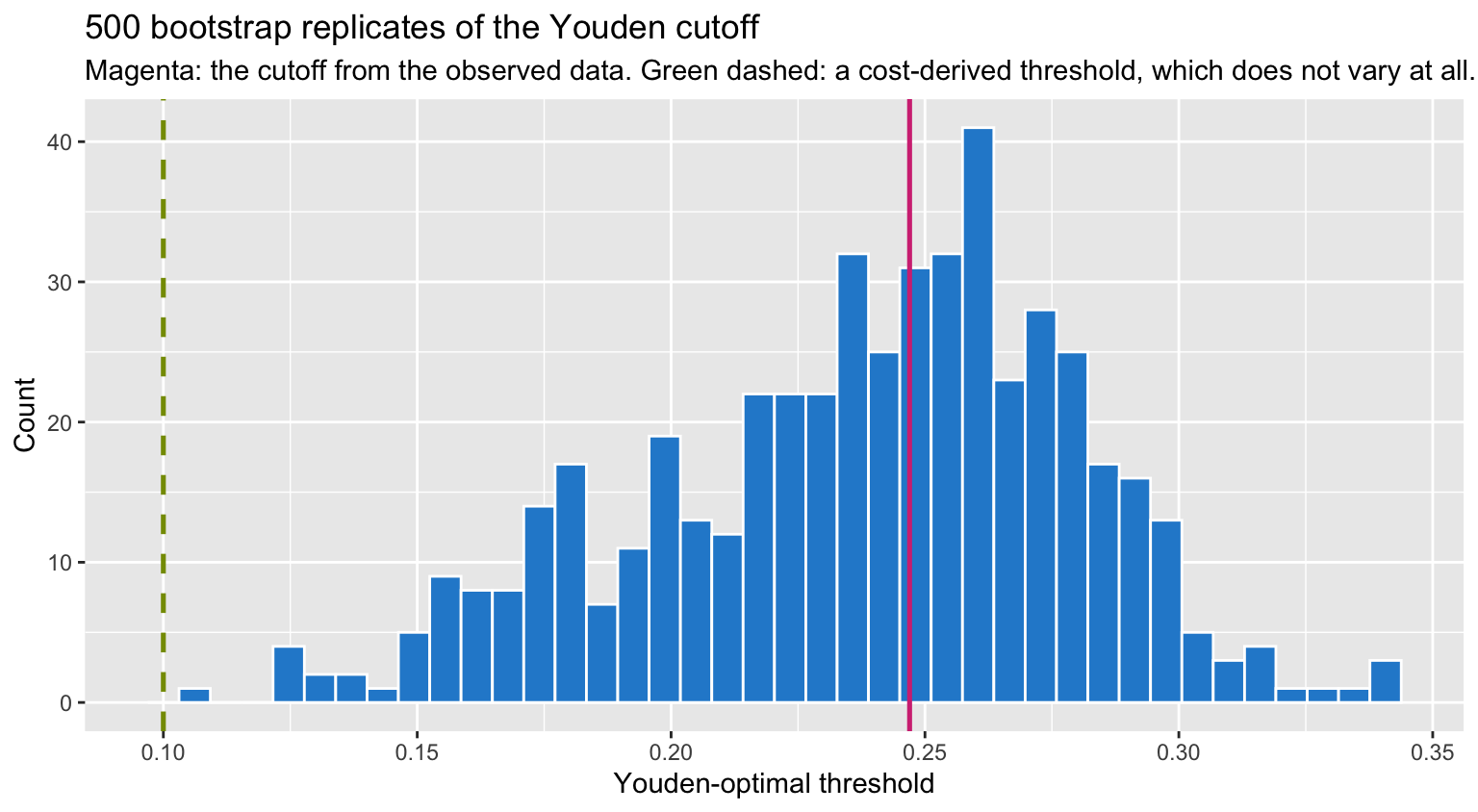
The interval spans a wide range of thresholds. A cost-derived threshold has no sampling variability whatsoever, because it is not estimated from the sample — it comes from the cost ratio you specify.
There is a second reason the empirical optimum is so unstable: the loss surface is nearly flat near its minimum, so noise moves the arg-min a long way while barely changing the loss.
data.frame(t = seq(0.35, 0.60, by = 0.05),
           loss = round(sapply(seq(0.35, 0.60, by = 0.05),
                               expected_loss, C_FP = 1, C_FN = 1), 4))
## t loss
## 1 0.35 0.177
## 2 0.40 0.168
## 3 0.45 0.173
## 4 0.50 0.171
## 5 0.55 0.169
## 6 0.60 0.169What this means in practice
The workflow this suggests is unglamorous:
- Fit by maximum likelihood and stop there as far as the model is concerned. No cutoff enters model building — Harrell’s “it is a mistake to consider thresholds when building a model” is the whole of it.
- Report the probabilities, and judge them with
measures that need no threshold: \(D_{xy}\), the \(c\)-index, Brier, pseudo-\(R^2\), and above all a calibration curve.
lrmprints these by default andvalidatede-optimises them. - If a decision must be made, get \(C_{FP}\) and \(C_{FN}\) from whoever owns the consequences and use \(p^* = C_{FP}/(C_{FP} + C_{FN})\). Different patients may well deserve different thresholds, and that is a feature.
- Do not tune the cutoff on the data. It is unstable, as the bootstrap shows, and it quietly substitutes the prevalence for your values.
The P-index of the original post has the same difficulty as Youden: PPV and NPV move with prevalence, so a threshold chosen to maximise them inherits the case mix of whatever sample you happened to collect. Harrell’s narrower objection also applies — PPV and NPV presume a binary test and no pre-test probability, when a fitted risk model gives you the posterior probability directly.
Youden still has a legitimate use. As a summary of a diagnostic test’s separation, independent of any decision, \(J\) is a reasonable one-number description, and it is honest about being prevalence-anchored. The error is reading “optimal cutoff” as though it were optimal for a decision. It is optimal for one cost ratio — the one your prevalence happens to imply.
References
- Gneiting T, Raftery AE. Strictly proper scoring rules, prediction, and estimation. JASA 2007;102:359–378.
- Harrell FE. Regression Modeling Strategies, 2nd ed. Springer, 2015.
- Blythe R et al. JAMIA 2023; doi:10.1093/jamia/ocad042 — setting thresholds from an institutional utility function.