
Maximum likelihood: from first principles to logistic regression
Contents
- Probability and likelihood are not the same function
- Why the logarithm
- Score and information: the curve’s slope and curvature
- Finding the maximum: Newton–Raphson
- From one parameter to a regression
- A clinical toy dataset
- Fitting it Harrell’s way with
rms - Three ways to test the same thing
- What the likelihood does not tell you
- Closing
Probability and likelihood are not the same function
Suppose 20 patients undergo flexible bronchoscopy and 7 of them desaturate. The binomial density
\[P(Y = y \mid p) = \binom{n}{y} p^{y} (1-p)^{n-y}\]
can be read in two directions, and the difference is the whole idea.
Read as a probability, \(p\) is fixed and \(y\) varies: it tells you how often each possible count occurs. Read as a likelihood, \(y\) is fixed at what you actually observed and \(p\) varies: it tells you how well each candidate value of \(p\) accounts for the data you have. Same algebra, different argument.
The second reading is not a probability distribution. It does not integrate to one over \(p\), and it is not \(P(p \mid y)\) – that would need a prior. It is simply a measure of relative support, and Fisher’s proposal was to take its maximiser as the estimate.
y <- 7; n <- 20

lik <- tibble(p = seq(0, 1, length.out = 801)) |>
  mutate(L = dbinom(y, n, p))

p_hat <- y / n

ggplot(lik, aes(p, L)) +
  geom_area(fill = pal[["blue"]], alpha = 0.18) +
  geom_line(colour = pal[["blue"]], linewidth = 0.9) +
  geom_vline(xintercept = p_hat, linetype = "dashed",
             colour = pal[["orange"]], linewidth = 0.7) +
  annotate("point", x = p_hat, y = dbinom(y, n, p_hat),
           colour = pal[["orange"]], size = 3) +
  annotate("text", x = p_hat + 0.03, y = dbinom(y, n, p_hat),
           label = expression(hat(p) == 0.35), hjust = 0, size = 4,
           colour = pal[["orange"]]) +
  labs(title = "Likelihood of p, having observed 7 desaturations in 20",
       subtitle = "the data are fixed; the parameter varies",
       x = "p (probability of desaturation)",
       y = "L(p) = P(Y = 7 | p)")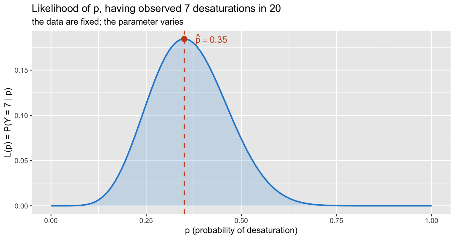
The curve peaks at 0.35, which is just \(y/n\). That is reassuring but not very informative – the interesting part is the shape.
Note also the integral:
integrate(function(p) dbinom(y, n, p), 0, 1)$value## [1] 0.04761905It is \(1/(n+1)\), not 1. The likelihood is a function of the parameter, not a density over it.
Why the logarithm
Nobody maximises the likelihood itself. Three reasons, in increasing order of importance.
First, arithmetic. With independent observations the likelihood is a product, and a product of 600 numbers below 1 underflows to zero in double precision. The log turns it into a sum.
Second, the maximiser is unchanged – \(\log\) is strictly increasing, so \(\arg\max L = \arg\max \log L\).
Third, and the real reason: the log-likelihood is the function that is approximately quadratic. All the standard machinery – standard errors, Wald tests, likelihood ratio tests, the whole asymptotic apparatus – is built on that quadratic shape. On the raw likelihood scale it is not there.
ll <- tibble(p = seq(0.02, 0.98, length.out = 801)) |>
  mutate(logL = dbinom(y, n, p, log = TRUE))

ggplot(ll, aes(p, logL)) +
  geom_line(colour = pal[["blue"]], linewidth = 0.9) +
  geom_vline(xintercept = p_hat, linetype = "dashed",
             colour = pal[["orange"]], linewidth = 0.7) +
  annotate("point", x = p_hat, y = dbinom(y, n, p_hat, log = TRUE),
           colour = pal[["orange"]], size = 3) +
  coord_cartesian(ylim = c(-15, 0)) +
  labs(title = "The same information on the log scale",
       subtitle = "a single smooth maximum, and near it, a parabola",
       x = "p", y = expression(log~L(p)))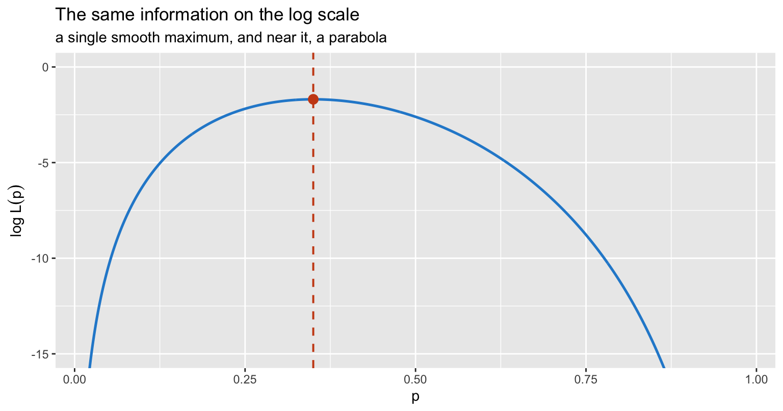
Score and information: the curve’s slope and curvature
Two derivatives carry everything.
The score is the first derivative of the log-likelihood:
\[U(p) = \frac{\partial \log L}{\partial p} = \frac{y}{p} - \frac{n-y}{1-p}\]
Setting it to zero gives the MLE. Here that is immediate: \(y(1-p) = (n-y)p\), so \(\hat p = y/n\).
The observed information is minus the second derivative:
\[I(p) = -\frac{\partial^2 \log L}{\partial p^2} = \frac{y}{p^2} + \frac{n-y}{(1-p)^2}\]
which at \(\hat p\) simplifies to \(n / (\hat p (1 - \hat p))\). Its reciprocal is the variance of the estimate, so
\[\mathrm{SE}(\hat p) = \sqrt{\frac{\hat p (1-\hat p)}{n}}\]
the familiar formula, derived rather than remembered. The interpretation is geometric: a sharply curved log-likelihood means the data strongly discriminate between nearby parameter values, which is exactly what a small standard error means.
score <- function(p) y/p - (n - y)/(1 - p)
info  <- function(p) y/p^2 + (n - y)/(1 - p)^2

c(score_at_mle = score(p_hat),
  info_at_mle  = info(p_hat),
  se_from_info = sqrt(1/info(p_hat)),
  se_textbook  = sqrt(p_hat * (1 - p_hat) / n))
## score_at_mle info_at_mle se_from_info se_textbook
## 0.0000000 87.9120879 0.1066536 0.1066536The quadratic approximation
Near the maximum, a second-order Taylor expansion gives
\[\log L(p) \approx \log L(\hat p) - \tfrac{1}{2} I(\hat p) (p - \hat p)^2\]
How good is that? It depends entirely on which scale you work on. Below, the same model is expanded on the probability scale and on the log-odds scale \(\beta = \log\{p/(1-p)\}\), where \(\log L(\beta) = y\beta - n\log(1 + e^{\beta})\) and \(I(\hat\beta) = n \hat p (1 - \hat p)\).
b_hat <- qlogis(p_hat)
ll_max <- dbinom(y, n, p_hat, log = TRUE)

# The two scales must carry the SAME additive constant or the panels will not
# be comparable: dbinom(log = TRUE) includes lchoose(n, y), the logit-scale
# kernel y*b - n*log(1 + e^b) does not. Omitting it shifts the log-odds curve
# down by lchoose(20, 7) = 11.26 and pushes it clean off the panel.
ll_b <- function(b) lchoose(n, y) + y * b - n * log1p(exp(b))

lv <- c("probability scale  (p)", "log-odds scale  (logit p)")

grid_p <- tibble(x = seq(0.10, 0.70, length.out = 400)) |>
  mutate(exact  = dbinom(y, n, x, log = TRUE),
         approx = ll_max - 0.5 * info(p_hat) * (x - p_hat)^2,
         scale  = factor(lv[1], levels = lv))

grid_b <- tibble(x = seq(qlogis(0.10), qlogis(0.70), length.out = 400)) |>
  mutate(exact  = ll_b(x),
         approx = ll_max - 0.5 * n * p_hat * (1 - p_hat) * (x - b_hat)^2,
         scale  = factor(lv[2], levels = lv))

both <- bind_rows(grid_p, grid_b)

long <- bind_rows(
  transmute(both, scale, x, value = exact,  curve = "exact log-likelihood"),
  transmute(both, scale, x, value = approx, curve = "quadratic approximation")
)

ggplot(long, aes(x, value, colour = curve, linetype = curve)) +
  geom_line(linewidth = 0.9) +
  facet_wrap(~ scale, scales = "free_x") +
  scale_colour_manual(values = unname(pal[c("blue", "magenta")])) +
  scale_linetype_manual(values = c("solid", "longdash")) +
  coord_cartesian(ylim = c(ll_max - 8, ll_max + 0.4)) +
  labs(title = "The quadratic approximation is a property of the scale, not the model",
       subtitle = "the approximation errs on both scales, but far less in the log-odds",
       x = NULL, y = "log-likelihood", colour = NULL, linetype = NULL) +
  theme(legend.position = "top")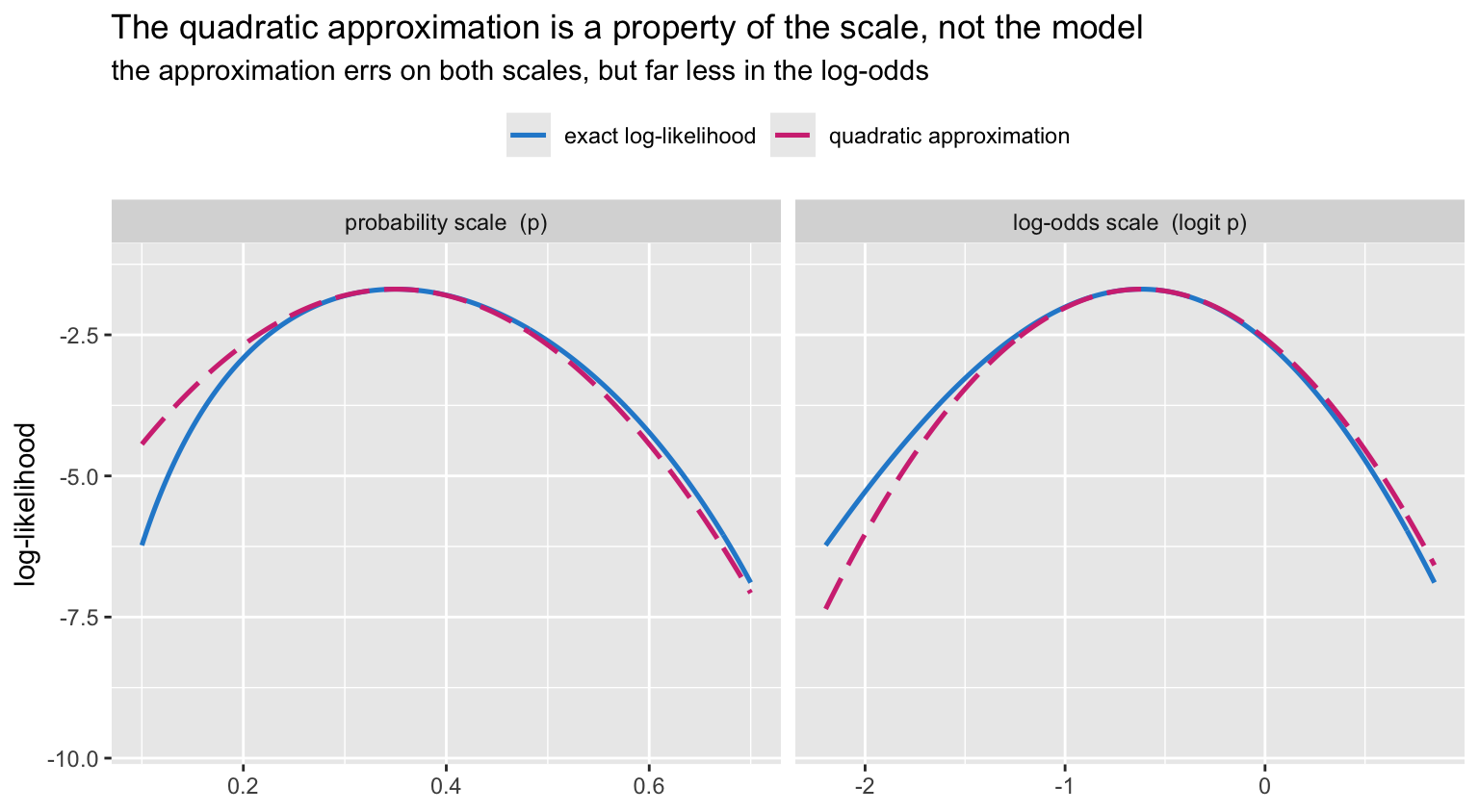
Both panels show some error, so it is worth measuring rather than eyeballing. A parabola is symmetric about its apex; the log-likelihood need not be. Compare how much height is lost two standard errors below the maximum with how much is lost two standard errors above:
se_p <- sqrt(p_hat * (1 - p_hat) / n)
se_b <- sqrt(1 / (n * p_hat * (1 - p_hat)))

drop_p <- dbinom(y, n, p_hat + c(-2, 2) * se_p, log = TRUE) - ll_max
drop_b <- ll_b(b_hat + c(-2, 2) * se_b) - ll_max

c(p_scale_gap = abs(diff(drop_p)), logodds_gap = abs(diff(drop_b))) |> round(3)
## p_scale_gap logodds_gap
## 1.053 0.348A perfectly quadratic log-likelihood would give a gap of zero. The log-odds scale is about three times closer to that ideal, and the advantage grows as \(\hat p\) moves away from 0.5.
The probability scale also has a harder failure mode. With 2 events in 20, \(\hat p \pm 2\,\mathrm{SE}\) reaches below zero – the Wald interval leaves the parameter space entirely:
ph2 <- 2 / 20
ph2 + c(-1, 1) * qnorm(0.975) * sqrt(ph2 * (1 - ph2) / 20)
## [1] -0.03147838 0.23147838The log-odds scale cannot do that: \(\mathrm{logit}^{-1}\) maps the whole real line into \((0, 1)\), so every interval comes back as a valid probability.
That is the real argument for parameterising logistic regression in log-odds. It is not that log-odds are intuitive – they are not. It is that the likelihood is close to Gaussian there and the parameter is unbounded, so symmetric Wald intervals, the normal approximation and the delta method all behave. Transform back to the probability scale after doing the inference, never before.
Finding the maximum: Newton–Raphson
For the binomial the MLE is closed-form. For almost everything else it is not, and we climb to it. Newton–Raphson uses the local quadratic: at the current guess, fit a parabola using the score and the information, jump to that parabola’s apex, repeat.
\[\beta_{k+1} = \beta_k + I(\beta_k)^{-1} U(\beta_k)\]
score_b <- function(b) y - n * plogis(b)
info_b  <- function(b) n * plogis(b) * (1 - plogis(b))

b <- 1.0                 # a deliberately poor start: p = 0.73
path <- tibble(iter = 0, beta = b, logL = ll_b(b),
               score = score_b(b), step = NA_real_)

for (k in 1:5) {
  step <- score_b(b) / info_b(b)
  b    <- b + step
  path <- bind_rows(path,
    tibble(iter = k, beta = b, logL = ll_b(b),
           score = score_b(b), step = step))
}

path |> mutate(across(where(is.numeric), \(x) round(x, 6)))
## # A tibble: 6 × 5
## iter beta logL score step
## <dbl> <dbl> <dbl> <dbl> <dbl>
## 1 0 1 -8.01 -7.62 NA
## 2 1 -0.938 -1.91 1.37 -1.94
## 3 2 -0.598 -1.69 -0.0951 0.340
## 4 3 -0.619 -1.69 -0.00029 -0.0208
## 5 4 -0.619 -1.69 0 -0.000064
## 6 5 -0.619 -1.69 0 0Four steps. The score collapses from -7.62 to effectively zero, and
beta lands on \(\log(7/13)
=\) -0.619039 to six decimals.
curve_b <- tibble(beta = seq(-2.2, 1.4, length.out = 600)) |>
  mutate(logL = ll_b(beta))

ggplot(curve_b, aes(beta, logL)) +
  geom_line(colour = pal[["grey"]], linewidth = 0.8) +
  geom_hline(yintercept = ll_max, linetype = "dotted",
             colour = pal[["blue"]]) +
  geom_path(data = path, colour = pal[["orange"]],
            linewidth = 0.6, linetype = "dashed",
            arrow = arrow(length = unit(0.14, "cm"), type = "closed")) +
  geom_point(data = path, aes(fill = factor(iter)),
             shape = 21, colour = pal[["orange"]], size = 3.6, stroke = 0.7) +
  # iterations 2-5 land on top of one another, so the labels must be repelled
  ggrepel::geom_text_repel(
    data = path, aes(label = iter), colour = pal[["orange"]], size = 3.4,
    nudge_y = -1.1, direction = "both", seed = 1,
    segment.size = 0.25, segment.colour = "grey70",
    min.segment.length = 0.25, box.padding = 0.3, show.legend = FALSE) +
  scale_fill_grey(start = 1, end = 0.35, guide = "none") +
  labs(title = "Newton--Raphson climbing the log-likelihood",
       subtitle = "numbered by iteration; the first step overshoots, then it converges quadratically",
       x = expression(beta == logit(p)), y = "log-likelihood")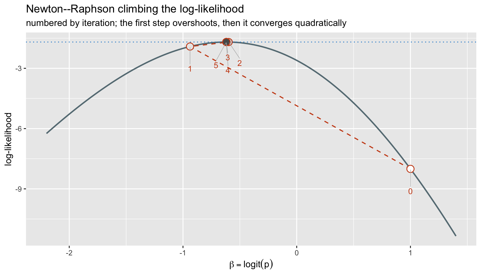
The first jump overshoots the maximum – the parabola fitted at \(p = 0.73\) is too narrow – but from there
convergence is quadratic, roughly doubling the number of correct digits
per step. glm() runs exactly this algorithm, dressed up as
iteratively reweighted least squares: each Newton step for a generalised
linear model can be written as a weighted least-squares fit, which is
why the output reports a working weight matrix rather than a
Hessian.
From one parameter to a regression
Nothing conceptual changes when \(p\) becomes a function of covariates. We model
\[\log \frac{p_i}{1 - p_i} = x_i^{\top}\beta, \qquad p_i = \mathrm{logit}^{-1}(x_i^{\top}\beta)\]
and the Bernoulli log-likelihood becomes
\[\log L(\beta) = \sum_i \left\{ y_i x_i^{\top}\beta - \log\left(1 + e^{x_i^{\top}\beta}\right) \right\}\]
The score and information generalise to a vector and a matrix:
\[U(\beta) = X^{\top}(y - p), \qquad I(\beta) = X^{\top} W X, \quad W = \mathrm{diag}\{p_i(1-p_i)\}\]
That is the whole of logistic regression. The score equations \(X^{\top}(y-p) = 0\) say the fitted probabilities must reproduce the observed totals in every direction spanned by the covariates, and \((X^{\top}WX)^{-1}\) is the covariance matrix of \(\hat\beta\).
The likelihood surface
With two parameters the log-likelihood is a surface, and the contours make the correlation between estimates visible.
set.seed(20261118)
nn   <- 600
agec <- round(rnorm(nn, 64, 11)) - 64
yy   <- rbinom(nn, 1, plogis(-1.1 + 0.035 * agec))

loglik2 <- function(b0, b1) {
  eta <- b0 + b1 * agec
  sum(yy * eta - log1p(exp(eta)))
}

fit2  <- glm(yy ~ agec, family = binomial)
mle2  <- coef(fit2)
llmax <- as.numeric(logLik(fit2))

surf <- expand.grid(b0 = seq(mle2[1] - 0.7, mle2[1] + 0.7, length.out = 140),
                    b1 = seq(mle2[2] - 0.045, mle2[2] + 0.045, length.out = 140)) |>
  as_tibble() |>
  rowwise() |>
  mutate(dev = 2 * (llmax - loglik2(b0, b1))) |>
  ungroup()

ggplot(surf, aes(b0, b1)) +
  geom_contour_filled(aes(z = dev),
                      breaks = c(0, 1, 2.3, 4, 6, 9.21, 14, 20, 30)) +
  geom_contour(aes(z = dev), breaks = qchisq(0.95, 2),
               colour = pal[["orange"]], linewidth = 0.9) +
  annotate("point", x = mle2[1], y = mle2[2], colour = "white",
           size = 3.2, shape = 4, stroke = 1.4) +
  scale_fill_ordinal(name = "deviance from\nthe maximum") +
  labs(title = "Log-likelihood surface for a two-parameter logistic model",
       subtitle = "heavy line = joint 95% region; x marks the MLE",
       x = expression(beta[0]~"(intercept)"),
       y = expression(beta[1]~"(age, centred)"))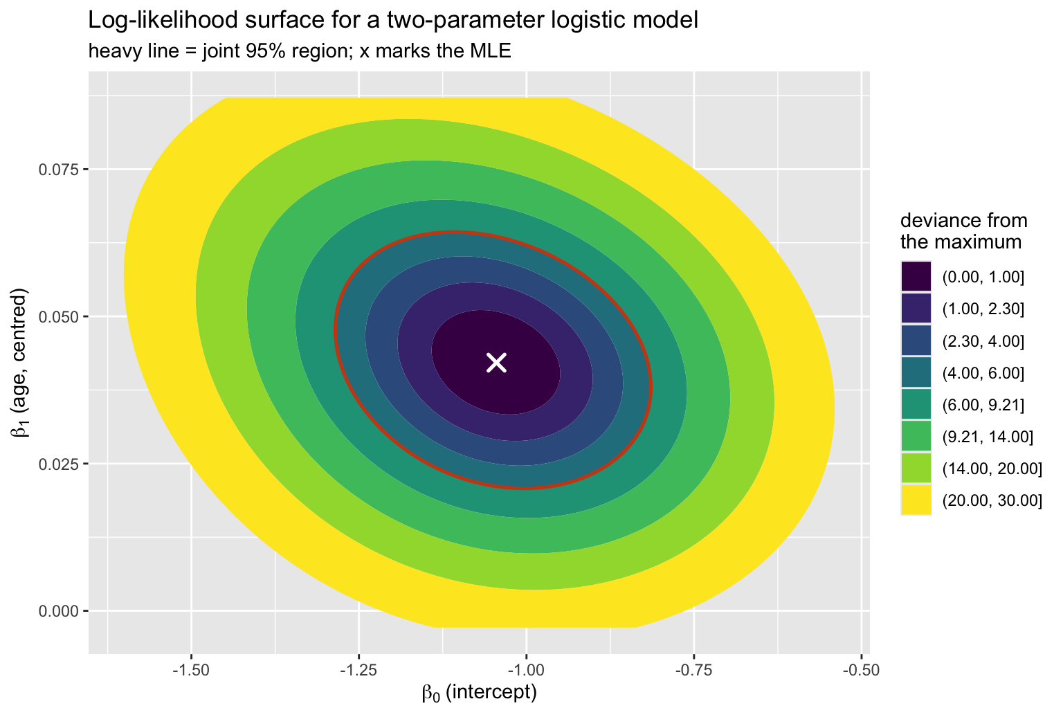
The contours are only slightly tilted, and that is because age was centred at 64 before fitting. The tilt is the correlation between the two estimates:
fit_raw <- glm(yy ~ I(agec + 64), family = binomial)
c(centred = cov2cor(vcov(fit2))[1, 2],
  raw_age = cov2cor(vcov(fit_raw))[1, 2]) |> round(3)
## centred raw_age
## -0.222 -0.988Centred, the estimates are nearly independent. On the raw age scale the correlation is almost \(-1\), and the same 95% region becomes a thin diagonal sliver: raising the slope and lowering the intercept to compensate leaves the fit essentially unchanged, so the data cannot separate the two. The likelihood there is a long flat ridge rather than a well-defined peak.
This is worth internalising, because it is the same geometry that produces alarming standard errors from uncentred polynomial and interaction terms. The fit is identical – predictions, deviance and \(C\) do not move – but the parameterisation is badly conditioned, and the information matrix is close to singular.
A clinical toy dataset
Something concrete to fit: 600 simulated bronchoscopies with desaturation as the outcome. The data-generating truth gives FEV1 a deliberately curved effect – risk is high and flat in severe obstruction, falls steeply through the middle of the range, then flattens again at normal lung function – plus a linear age effect, a sex effect, and BMI as a genuine null variable.
set.seed(20261118)
n_pt <- 600

age  <- round(rnorm(n_pt, 64, 11))
sex  <- factor(sample(c("female", "male"), n_pt, TRUE, prob = c(0.45, 0.55)))
fev1 <- round(pmin(125, pmax(25, rnorm(n_pt, 78, 18))))
bmi  <- round(rnorm(n_pt, 27.5, 4.5), 1)

# A sigmoid in fev1, not a quadratic. A quadratic whose vertex falls inside the
# observed range would make risk *fall* again at very low FEV1 - clinically
# backwards, however convenient the algebra.
eta <- -1.9 + 0.032 * (age - 64) + 0.70 * (sex == "male") +
        2.2 * plogis(-(fev1 - 65) / 9) + 0.030 * (bmi - 27.5)

d <- tibble(hypox = rbinom(n_pt, 1, plogis(eta)),
            age, sex, fev1, bmi)

d
## # A tibble: 600 × 5
## hypox age sex fev1 bmi
## <int> <dbl> <fct> <dbl> <dbl>
## 1 0 63 male 70 20.6
## 2 1 76 female 76 28.2
## 3 1 59 female 51 28.4
## 4 0 65 male 123 20.6
## 5 1 75 male 51 24.1
## 6 1 77 male 84 32.9
## 7 0 68 female 85 24.2
## 8 0 72 female 97 26.1
## 9 1 67 female 59 19.7
## 10 0 82 male 98 30.1
## # ℹ 590 more rowsc(events = sum(d$hypox), n = nrow(d), prevalence = mean(d$hypox))## events n prevalence
## 187.0000000 600.0000000 0.3116667187 events. Harrell’s rule of thumb is roughly 15 events per candidate parameter before you can trust a model without penalisation; with 187 events we can afford the six parameters below, but not many more, and certainly not a round of stepwise selection on top.
ggplot(d, aes(fev1, hypox)) +
  geom_point(aes(colour = sex), alpha = 0.35,
             position = position_jitter(height = 0.035, width = 0.4)) +
  geom_smooth(method = "loess", span = 0.9, se = TRUE,
              colour = pal[["magenta"]], fill = pal[["magenta"]],
              alpha = 0.15, linewidth = 0.9) +
  scale_colour_manual(values = unname(pal[c("blue", "green")])) +
  labs(title = "Desaturation against FEV1 (% predicted)",
       subtitle = "a nonparametric smoother, before any model is imposed",
       x = "FEV1 (% predicted)", y = "desaturation (jittered)",
       colour = NULL)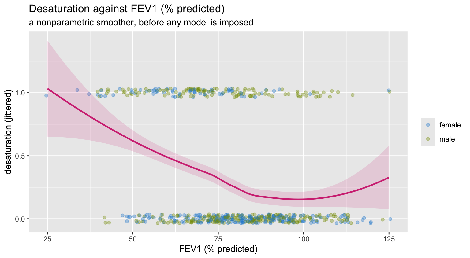
The smoother bends. A model with fev1 entered linearly
would be fitting a straight line through that.
Fitting it Harrell’s way with rms
Three things distinguish the rms idiom from a bare
glm() call.
Flexibility by default. A continuous predictor goes in as a restricted cubic spline unless there is a reason to force linearity. Four knots costs three degrees of freedom and buys the ability to detect curvature instead of assuming it away. The restriction – linear beyond the outer knots – keeps the tails from flying off.
datadist. rms stores the
distribution of every predictor up front, so that later calls know what
“holding the other variables fixed” should mean (medians for continuous,
modes for categorical) and what range to plot over.
Everything downstream for free. One fit object
supports anova, summary, Predict,
validate, calibrate and nomogram
without repeating yourself.
# rms stores only the NAME of the datadist object and looks it up in the global
# environment. knitr evaluates each chunk in its own environment, so inside an
# .Rmd this assignment is required - without it lrm() fails with
# "dataset dd not found for options(datadist=)".
dd <- datadist(d)
assign("dd", dd, envir = globalenv())
options(datadist = "dd")

f <- lrm(hypox ~ rcs(fev1, 4) + age + sex + bmi,
         data = d, x = TRUE, y = TRUE)
f
## Logistic Regression Model
##
## lrm(formula = hypox ~ rcs(fev1, 4) + age + sex + bmi, data = d,
## x = TRUE, y = TRUE)
##
## Model Likelihood Discrimination Rank Discrim.
## Ratio Test Indexes Indexes
## Obs 600 LR chi2 103.63 R2 0.223 C 0.751
## 0 413 d.f. 6 R2(6,600)0.150 Dxy 0.501
## 1 187 Pr(> chi2) <0.0001 R2(6,386.2)0.223 gamma 0.501
## max |deriv| 4e-05 Brier 0.180 tau-a 0.215
##
## Coef S.E. Wald Z Pr(>|Z|)
## Intercept -0.3565 1.4155 -0.25 0.8011
## fev1 -0.0469 0.0191 -2.45 0.0142
## fev1' -0.0577 0.0565 -1.02 0.3069
## fev1'' 0.4486 0.2538 1.77 0.0772
## age 0.0377 0.0091 4.13 <0.0001
## sex=male 0.9473 0.2023 4.68 <0.0001
## bmi 0.0124 0.0210 0.59 0.5541max |deriv| in that header is the largest absolute
element of the score vector at the reported solution. It should be a
very small number: it is rms telling you the optimiser
genuinely reached a stationary point rather than stopping somewhere near
one. Section 3 is what that line is reporting on.
The Wald table from anova.rms is organised by
predictor, not by coefficient, which is what you want once a
variable occupies several columns of the design matrix. The
Nonlinear line is the joint test of the two spline terms
beyond the linear one.
ad <- as.data.frame(unclass(anova(f)))
names(ad) <- c("chisq", "df", "p")

ad_plot <- ad |>
  tibble::rownames_to_column("term") |>
  filter(term != "TOTAL") |>
  mutate(nonlinear = grepl("Nonlinear", term),
         term  = trimws(term),
         label = ifelse(nonlinear, "fev1: nonlinear component", term),
         stat  = chisq - df)

ggplot(ad_plot, aes(stat, reorder(label, stat))) +
  geom_segment(aes(xend = 0, yend = reorder(label, stat)),
               colour = pal[["grey"]], linewidth = 0.5) +
  geom_point(aes(colour = nonlinear), size = 4) +
  scale_colour_manual(values = unname(pal[c("blue", "magenta")]),
                      guide = "none") +
  labs(title = "Relative predictive strength",
       subtitle = expression(Wald~chi^2~minus~its~degrees~of~freedom),
       x = NULL, y = NULL)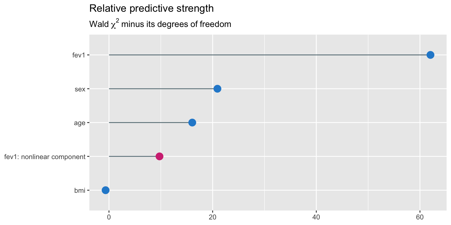
Subtracting the degrees of freedom is Harrell’s device for making a 3-df spline comparable with a 1-df binary term: it is the chi-square penalised by what it cost to get. FEV1 dominates by a wide margin, age and sex are real but modest, and BMI sits at the bottom – correctly, since we generated it as noise.
Partial effects
Predict() varies one predictor across its observed range
while holding the others at their datadist reference
values. It returns a plain data frame, so the plotting is ordinary
ggplot work.
pr <- as.data.frame(Predict(f, fev1, fun = plogis))

ggplot(pr, aes(fev1, yhat)) +
  geom_ribbon(aes(ymin = lower, ymax = upper),
              fill = pal[["blue"]], alpha = 0.20) +
  geom_line(colour = pal[["blue"]], linewidth = 1) +
  geom_rug(data = d, aes(x = fev1, y = NULL), sides = "b",
           alpha = 0.25, colour = pal[["grey"]]) +
  scale_y_continuous(labels = scales::percent) +
  labs(title = "Fitted risk of desaturation across FEV1",
       subtitle = "restricted cubic spline, 4 knots; other predictors at their reference values",
       x = "FEV1 (% predicted)", y = "probability of desaturation")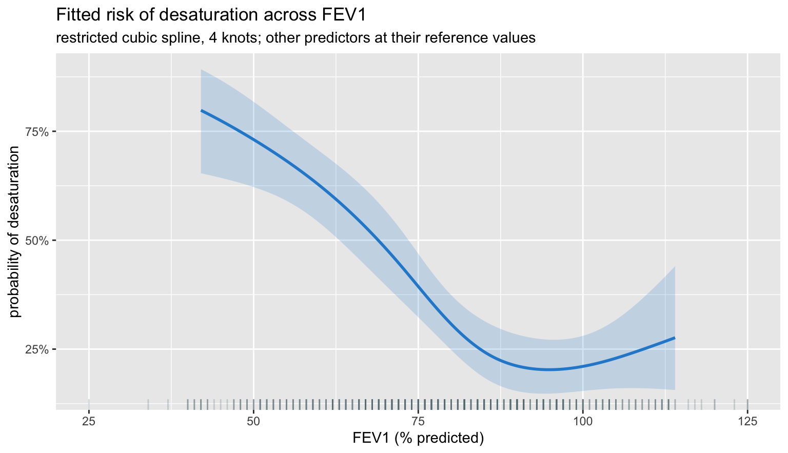
The spline recovers the shape we built in: a high plateau below roughly 55% predicted, a steep fall through the middle of the range, and a low plateau above about 90%. A linear term would have averaged those three regimes into a single slope that is wrong in all of them.
It also does something we did not build in. Above about 100% predicted the fitted curve turns upward again. There is no such effect in the data-generating model – it is the spline chasing noise where there is very little data, and the honest signal that this is happening is the ribbon, which balloons over exactly that stretch. Read the band, not the line.
Two things widen it in the tails. The information matrix \(X^{\top}WX\) is thin on observations there; and \(W = p(1-p)\) shrinks as fitted probabilities approach 0 or 1, so each extreme patient contributes less information than their rarity alone would suggest. This is the practical argument for not reading spline fits beyond the inner knots, and for preferring fewer knots when events are scarce.
one_var <- function(var) {
  as.data.frame(Predict(f, name = var, fun = plogis)) |>
    transmute(x = .data[[var]], yhat, lower, upper, var = var)
}

grid_all <- bind_rows(lapply(c("fev1", "age", "bmi"), one_var))

ggplot(grid_all, aes(x, yhat)) +
  geom_ribbon(aes(ymin = lower, ymax = upper),
              fill = pal[["blue"]], alpha = 0.18) +
  geom_line(colour = pal[["blue"]], linewidth = 0.9) +
  facet_wrap(~ var, scales = "free_x") +
  scale_y_continuous(labels = scales::percent) +
  labs(title = "All continuous partial effects on one page",
       subtitle = "age is linear by specification; bmi is flat because it is noise",
       x = NULL, y = "probability of desaturation")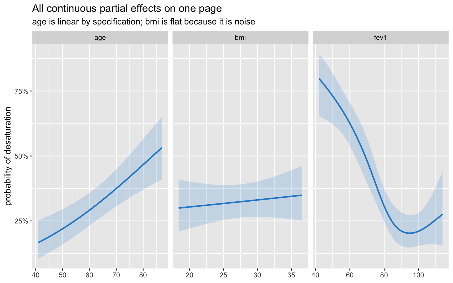
Effect sizes as odds ratios
summary.rms reports an inter-quartile-range effect by
default rather than a per-unit one. For a spline term a per-unit odds
ratio would be meaningless – the slope is different everywhere – so the
question becomes “how much does risk change between a typical low and a
typical high value”, which is what the IQR contrast answers.
sm   <- unclass(summary(f))
keep <- which(sm[, "Type"] == 2)          # the odds-ratio rows

or <- tibble(term = trimws(rownames(sm)[keep - 1]),
             low  = sm[keep, "Low"],
             high = sm[keep, "High"],
             or   = sm[keep, "Effect"],
             lo   = sm[keep, "Lower 0.95"],
             hi   = sm[keep, "Upper 0.95"]) |>
  mutate(label = sprintf("%s  (%g to %g)", term, low, high))

ggplot(or, aes(or, reorder(label, or))) +
  geom_vline(xintercept = 1, linetype = "dashed", colour = pal[["grey"]]) +
  geom_pointrange(aes(xmin = lo, xmax = hi), colour = pal[["blue"]],
                  linewidth = 0.7, size = 0.6) +
  scale_x_log10() +
  labs(title = "Inter-quartile-range odds ratios",
       subtitle = "log scale, so that an odds ratio and its reciprocal are equidistant from 1",
       x = "odds ratio", y = NULL)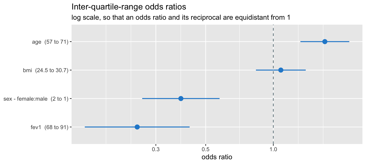
The log scale is not decoration. Odds ratios are multiplicative, their sampling distribution is symmetric on the log scale, and only there does an OR of 2 look like the same amount of evidence as an OR of 0.5.
Three ways to test the same thing
Having a likelihood gives three asymptotically equivalent tests, which differ in what they require and in how they behave at finite sample size.
| Test | What it uses | Needs |
|---|---|---|
| Wald | curvature at \(\hat\beta\) | one fit |
| Likelihood ratio | height difference between maxima | two fits |
| Score | slope at the null | one fit, under \(H_0\) |
The Wald test is cheapest and the least trustworthy: it reads the
curvature only at the maximum, so a skewed log-likelihood misleads it.
The likelihood ratio test compares the actual heights and is the one to
prefer. Harrell’s lrtest() does it directly.
f_lin <- lrm(hypox ~ fev1 + age + sex + bmi, data = d)   # force linearity
lrtest(f_lin, f)
##
## Model 1: hypox ~ fev1 + age + sex + bmi
## Model 2: hypox ~ rcs(fev1, 4) + age + sex + bmi
##
## L.R. Chisq d.f. P
## 10.693405157 2.000000000 0.004763833Compare that with the Wald Nonlinear row from
anova(f):
nl <- ad[grepl("Nonlinear", rownames(ad)), ]
c(wald_chisq = nl$chisq, wald_p = nl$p)
## wald_chisq wald_p
## 11.749642609 0.002809296Same conclusion here, different numbers. When they disagree materially, believe the likelihood ratio.
Profile likelihood
The honest confidence interval for a single coefficient comes from the likelihood itself: fix that coefficient at a candidate value, re-maximise over all the others, and record how much log-likelihood you had to give up. Keep the values that cost less than \(\chi^2_{1,0.95}/2 = 1.92\).
The re-maximisation is done by pushing the fixed term into the
offset.
X  <- model.matrix(~ rcs(fev1, 4) + age + sex + bmi, data = d)
j  <- which(colnames(X) == "age")
b_age  <- coef(f)[["age"]]
se_age <- sqrt(diag(vcov(f)))[["age"]]

prof_ll <- function(b) {
  m <- glm.fit(X[, -j, drop = FALSE], d$hypox,
               offset = b * X[, j], family = binomial())
  -m$deviance / 2            # for 0/1 data the saturated log-likelihood is 0
}

ll_full <- -f$deviance[2] / 2

prof <- tibble(b = seq(b_age - 4 * se_age, b_age + 4 * se_age,
                       length.out = 241)) |>
  rowwise() |>
  mutate(profile = 2 * (ll_full - prof_ll(b))) |>
  ungroup() |>
  mutate(wald = ((b - b_age) / se_age)^2)

prof_long <- bind_rows(
  transmute(prof, b, value = profile, curve = "profile deviance"),
  transmute(prof, b, value = wald,    curve = "Wald (quadratic)")
)

cut <- qchisq(0.95, 1)

ggplot(prof_long, aes(b, value, colour = curve, linetype = curve)) +
  geom_line(linewidth = 0.9) +
  geom_hline(yintercept = cut, colour = pal[["orange"]],
             linetype = "dotted", linewidth = 0.7) +
  annotate("text", x = b_age - 4 * se_age, y = cut + 0.55, hjust = 0,
           label = "chi-squared(1) 95% cutoff = 3.84", size = 3.4,
           colour = pal[["orange"]]) +
  scale_colour_manual(values = unname(pal[c("blue", "magenta")])) +
  scale_linetype_manual(values = c("solid", "longdash")) +
  coord_cartesian(ylim = c(0, 16)) +
  labs(title = "Profile deviance for the age coefficient",
       subtitle = "where the curves separate, the Wald interval is the wrong one",
       x = expression(beta[age]), y = "deviance from the maximum",
       colour = NULL, linetype = NULL) +
  theme(legend.position = "top")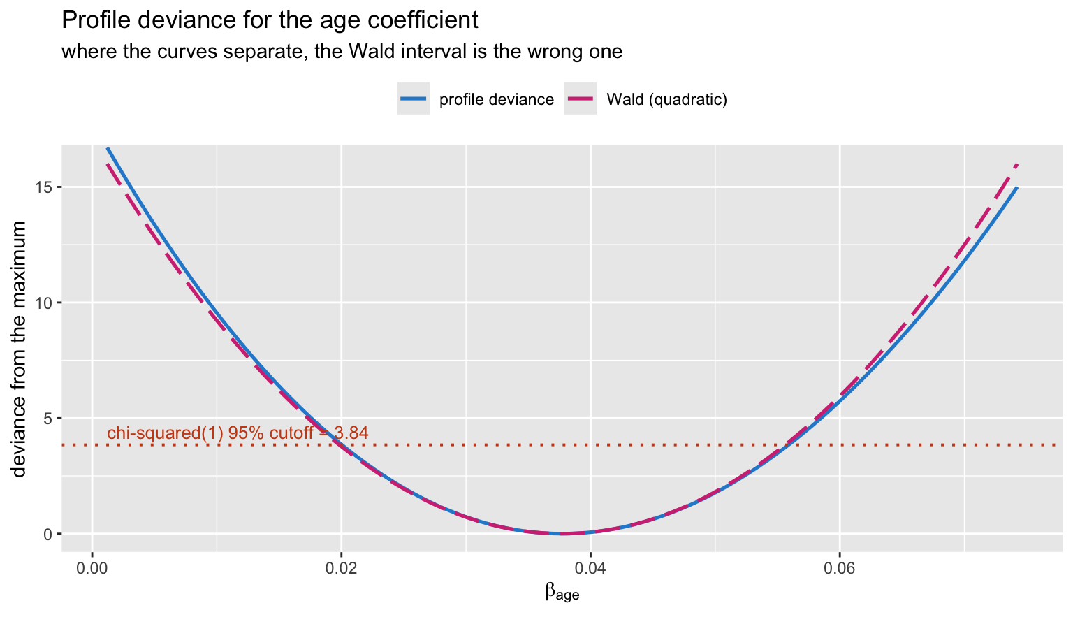
root <- function(lo, hi) {
  uniroot(function(b) 2 * (ll_full - prof_ll(b)) - cut,
          lower = lo, upper = hi, tol = 1e-8)$root
}

rbind(profile = c(root(b_age - 6*se_age, b_age), root(b_age, b_age + 6*se_age)),
      wald    = b_age + c(-1, 1) * qnorm(0.975) * se_age) |>
  round(4)
## [,1] [,2]
## profile 0.0200 0.0559
## wald 0.0198 0.0556With 187 events and a well-behaved predictor the two intervals nearly coincide – the quadratic approximation is doing its job. The divergence grows with small samples, sparse cells and coefficients near the boundary of separation, and the profile version is the one that stays correct.
What the likelihood does not tell you
Maximum likelihood answers one question: which parameter values best account for this dataset. It says nothing about how the model will do on the next one. The apparent \(C\) of 0.751 is an in-sample number, and it is optimistic by construction.
validate() quantifies that optimism by bootstrap: refit
on each resample, evaluate on the original data, and average the
gap.
set.seed(314)
v <- validate(f, B = 300)
round(v[c("Dxy", "R2", "Slope", "Emax"), ], 4)
## index.orig training test optimism index.corrected Lower Upper n
## Dxy 0.5011 0.5102 0.4881 0.0221 0.4790 0.3951 0.5581 300
## R2 0.2231 0.2342 0.2135 0.0207 0.2024 0.1277 0.2697 300
## Slope 1.0000 1.0000 0.9470 0.0530 0.9470 0.7102 1.2051 300
## Emax 0.0000 0.0000 0.0407 -0.0407 0.0407 -0.0082 0.1115 300dxy_corr <- v["Dxy", "index.corrected"]
c(C_apparent = f$stats[["C"]], C_corrected = dxy_corr / 2 + 0.5)## C_apparent C_corrected
## 0.7505406 0.7394880The corrected Slope below 1 is the calibration-slope
shrinkage: the model’s predictions are slightly too extreme, exactly the
overfitting you would expect from estimating six parameters from 187
events.
set.seed(315)
cal <- calibrate(f, B = 300)

cal_df <- as.data.frame(unclass(cal)[, c("predy", "calibrated.orig",
                                         "calibrated.corrected")])

cal_long <- bind_rows(
  transmute(cal_df, predy, actual = calibrated.orig,
            curve = "apparent"),
  transmute(cal_df, predy, actual = calibrated.corrected,
            curve = "bias-corrected (bootstrap)")
)

ggplot(cal_long, aes(predy, actual, colour = curve, linetype = curve)) +
  geom_abline(slope = 1, intercept = 0, colour = pal[["grey"]],
              linetype = "dashed") +
  geom_line(linewidth = 0.9) +
  geom_rug(data = d, inherit.aes = FALSE,
           aes(x = predict(f, type = "fitted")), sides = "b",
           alpha = 0.2, colour = pal[["grey"]]) +
  scale_colour_manual(values = unname(pal[c("blue", "magenta")])) +
  scale_linetype_manual(values = c("solid", "longdash")) +
  scale_x_continuous(labels = scales::percent) +
  scale_y_continuous(labels = scales::percent) +
  coord_equal() +
  labs(title = "Calibration: predicted versus observed risk",
       subtitle = "dashed = perfect; the gap between the two curves is the optimism",
       x = "predicted probability", y = "observed proportion",
       colour = NULL, linetype = NULL) +
  theme(legend.position = "top")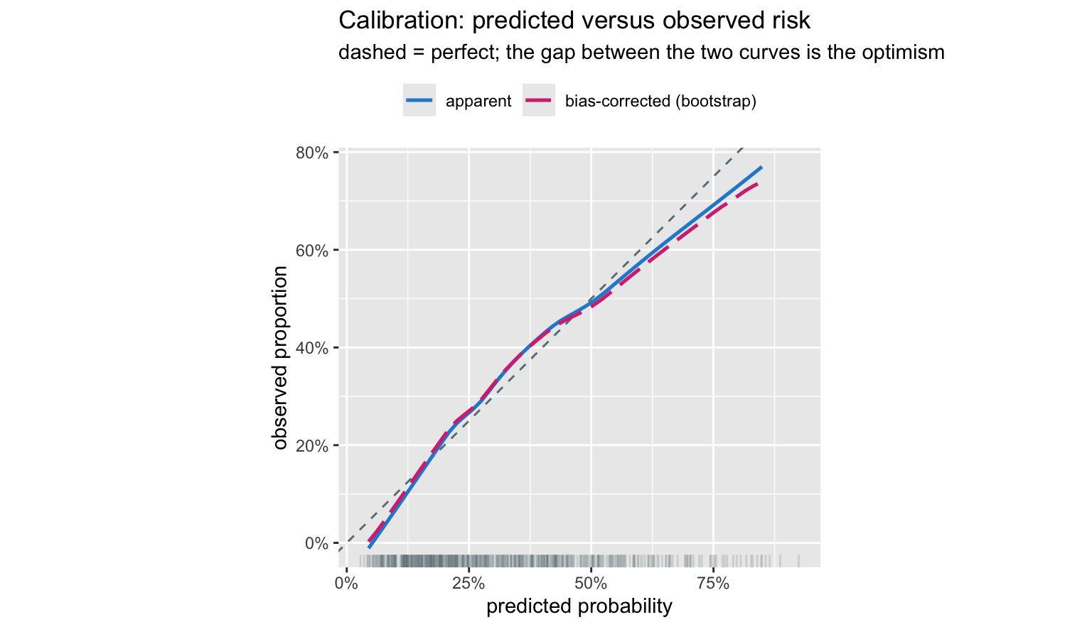
The vertical distance between the two curves is the
overfitting, made visible. Nothing in the likelihood could have shown
you that, because the likelihood was maximised on these same 600
patients. You need resampling, and rms makes it a
one-liner.
A calibration curve is also the right place to look before anyone starts talking about thresholds. A model that discriminates well but calibrates badly will produce decision rules that are wrong in a way that no choice of cutoff repairs – which is the subject of the companion post on MLE and the optimal classification threshold.
Closing
The thread running through all of this: the log-likelihood is a surface, its peak is the estimate, its curvature is the precision, and its height is the currency of model comparison. Everything else – score equations, standard errors, Wald and likelihood ratio tests, profile intervals, IRLS – is a statement about the geometry of that surface.
What that leaves out is equally worth stating. The likelihood is
maximised on the data in hand, so it cannot speak to out-of-sample
performance; it assumes the model class contains something reasonable;
and it is silent on the decision problem. rms is built
around those gaps: splines so the model class is wide enough,
validate and calibrate so the optimism is
measured rather than hoped away, and effects reported as interpretable
contrasts rather than raw coefficients.
References
- Harrell FE. Regression Modeling Strategies, 2nd ed. Springer, 2015. Chapters 9–10.
- Harrell FE. Biostatistics for Biomedical Research, hbiostat.org.
- Fisher RA. On the mathematical foundations of theoretical statistics. Phil Trans R Soc A 1922;222:309–368.
- Cox DR, Hinkley DV. Theoretical Statistics. Chapman & Hall, 1974. Chapter 9.
- Venzon DJ, Moolgavkar SH. A method for computing profile-likelihood-based confidence intervals. Appl Stat 1988;37:87–94.