
Frequentist, likelihood and Bayesian: three answers to one trial
Contents
Three different questions
The three traditions are usually taught as rival answers to one question. They are better understood as careful answers to three different questions.
| The question it answers | What is random | |
|---|---|---|
| Frequentist | If I follow this procedure forever, how often will it mislead me? | the data |
| Likelihood | How much better does this data fit one value than another? | nothing |
| Bayesian | Given what I knew before and what I have now seen, what should I believe? | the parameter |
An everyday version. You are waiting for a bus that is now 20 minutes late. The frequentist asks how often a working bus service produces a 20-minute gap, and if that is rare enough, declares the service broken. The likelihoodist asks how much better “the service is broken” explains a 20-minute gap than “the service is fine” – and reports the ratio, without declaring anything. The Bayesian notes that this line is reliable six days out of seven, combines that with the 20 minutes, and gives you the probability that today is the bad day. Only the third answers the question you actually care about, and only the third requires you to admit what you believed before you got to the stop.
The disagreements are mostly invisible when data are plentiful. They become sharp exactly where clinical research usually sits: small samples, borderline results.
One small trial
A single-centre randomised trial of high-flow nasal oxygen versus standard nasal cannula during flexible bronchoscopy. Outcome: any desaturation below 90% during the procedure. Forty patients per arm.
nc <- 40; yc <- 18     # standard cannula: 18 of 40 desaturated
nt <- 40; yt <-  9     # high-flow:         9 of 40 desaturated

pc_hat <- yc / nc
pt_hat <- yt / nt
rd_hat <- pt_hat - pc_hat          # risk difference, negative = benefit

c(standard = pc_hat, high_flow = pt_hat, risk_difference = rd_hat)
## standard high_flow risk_difference
## 0.450 0.225 -0.225arms <- tibble(
arm = factor(c("standard cannula", "high-flow"),
levels = c("standard cannula", "high-flow")),
y = c(yc, yt), n = c(nc, nt)) |>
mutate(p = y / n,
lo = mapply(\(a, b) binom.test(a, b)$conf.int[1], y, n),
hi = mapply(\(a, b) binom.test(a, b)$conf.int[2], y, n))
ggplot(arms, aes(p, arm)) +
geom_vline(xintercept = 0, colour = NA) +
geom_errorbar(aes(xmin = lo, xmax = hi), orientation = "y", width = 0.12,
colour = pal[["grey"]], linewidth = 0.7) +
geom_point(aes(colour = arm), size = 5) +
geom_text(aes(label = sprintf("%d/%d", y, n)), vjust = -1.6, size = 3.6,
colour = pal[["grey"]]) +
scale_colour_manual(values = unname(pal[c("orange", "blue")]),
guide = "none") +
scale_x_continuous(labels = scales::percent, limits = c(0, 0.75)) +
labs(title = "Desaturation during bronchoscopy",
subtitle = "exact binomial 95% intervals within each arm",
x = "proportion desaturating", y = NULL)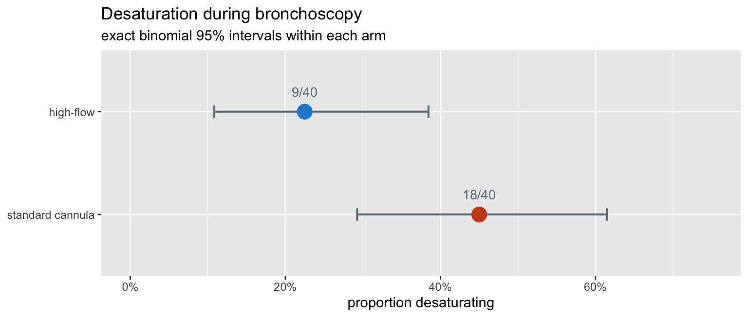
A 22.5 percentage-point absolute reduction. Now: is it real?
The frequentist answer
What a p-value actually is
A p-value is a statement about data that were never collected. It asks: if the two arms truly had the same risk, how often would an experiment like this one produce a difference at least as large as the one I saw?
We can simply do it. Simulate the trial many times under the null, with both arms sharing the pooled rate.
set.seed(2026)
p_pool <- (yc + yt) / (nc + nt)
M <- 100000

null_rd <- rbinom(M, nt, p_pool) / nt - rbinom(M, nc, p_pool) / nc
p_sim   <- mean(abs(null_rd) >= abs(rd_hat) - 1e-9)

c(pooled_rate = p_pool, simulated_two_sided_p = p_sim)
## pooled_rate simulated_two_sided_p
## 0.33750 0.04405nd <- tibble(rd = null_rd) |>
count(rd) |>
mutate(prop = n / sum(n),
tail = abs(rd) >= abs(rd_hat) - 1e-9)
ggplot(nd, aes(rd, prop, fill = tail)) +
geom_col(width = 0.022) +
geom_vline(xintercept = c(-1, 1) * abs(rd_hat), linetype = "dashed",
colour = pal[["orange"]], linewidth = 0.7) +
scale_fill_manual(values = unname(pal[c("grey", "orange")]),
labels = c("ordinary noise", "at least as extreme"),
name = NULL) +
scale_x_continuous(labels = scales::percent) +
labs(title = "What a p-value is: a tail area in a world where the drug does nothing",
subtitle = sprintf("100,000 simulated trials with both arms at the pooled rate of %.1f%%",
100 * p_pool),
x = "risk difference", y = "proportion of simulated trials") +
theme(legend.position = "top")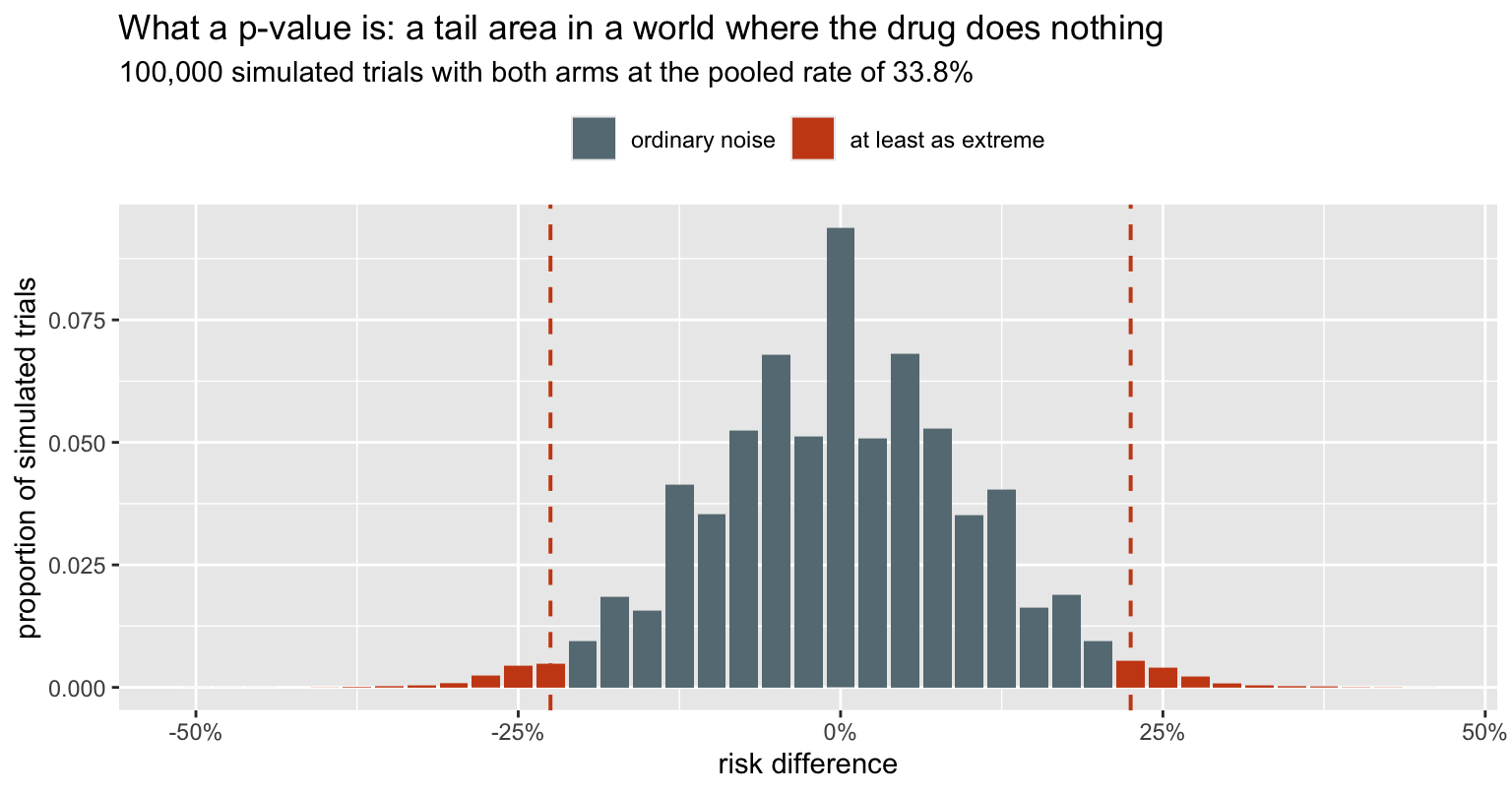
The shaded mass is the p-value, and it is 0.044 – which, as the next section shows, is yet another number, sitting between the exact and the uncorrected answers. Notice what the picture does not contain: any representation of the hypothesis that the treatment works. The p-value is computed entirely inside the null world. It cannot tell you the probability that the treatment works, because nothing in its construction refers to that.
Four p-values from one table
There is no such thing as the p-value for a 2x2 table. There are several, they rest on different approximations, and here they straddle 0.05.
# likelihood ratio (G-squared): compare the free fit with the pooled fit
ll_free <- yc*log(pc_hat) + (nc-yc)*log(1-pc_hat) +
           yt*log(pt_hat) + (nt-yt)*log(1-pt_hat)
ll_null <- (yc+yt)*log(p_pool) + (nc+nt-yc-yt)*log(1-p_pool)
G2      <- 2 * (ll_free - ll_null)

pvals <- tibble(
  test = c("Fisher exact",
           "chi-square, continuity-corrected",
           "chi-square, uncorrected",
           "likelihood ratio (G-squared)"),
  p = c(fisher.test(matrix(c(yt, nt-yt, yc, nc-yc), 2, byrow = TRUE))$p.value,
        prop.test(c(yt, yc), c(nt, nc))$p.value,
        prop.test(c(yt, yc), c(nt, nc), correct = FALSE)$p.value,
        pchisq(G2, 1, lower.tail = FALSE)))

pvals |> mutate(p = round(p, 4), verdict = ifelse(p < 0.05, "significant", "not"))
## # A tibble: 4 × 3
## test p verdict
## <chr> <dbl> <chr>
## 1 Fisher exact 0.0576 not
## 2 chi-square, continuity-corrected 0.0586 not
## 3 chi-square, uncorrected 0.0333 significant
## 4 likelihood ratio (G-squared) 0.0321 significantSame 80 patients, same table. Two tests say the result is significant and two say it is not, and the choice between them is a choice between approximations, not a choice about the biology. Any sentence of the form “the trial was negative” is hiding this.
What a confidence interval guarantees
A 95% confidence interval does not say there is a 95% probability that the true value lies inside it. It says: this procedure, repeated, produces intervals that cover the truth 95% of the time. The guarantee attaches to the method, not to the one interval you are holding.
That is a claim we can check directly. Fix a true risk difference, simulate trials, and count.
truth_c <- 0.45; truth_t <- 0.25        # a true risk difference of -0.20
truth_rd <- truth_t - truth_c

# cbind, not c: this has to stay a 2-column matrix when the inputs are vectors
wald_ci <- function(yt, nt, yc, nc, z = qnorm(0.975)) {
  pt <- yt/nt; pc <- yc/nc
  se <- sqrt(pt*(1-pt)/nt + pc*(1-pc)/nc)
  cbind(lo = pt - pc - z*se, hi = pt - pc + z*se)
}

set.seed(11)
R   <- 20000
sim <- tibble(yt = rbinom(R, nt, truth_t), yc = rbinom(R, nc, truth_c)) |>
  mutate(lo = wald_ci(yt, nt, yc, nc)[, "lo"],
         hi = wald_ci(yt, nt, yc, nc)[, "hi"],
         covers = lo <= truth_rd & truth_rd <= hi)

c(nominal = 0.95, actual_coverage = mean(sim$covers))
## nominal actual_coverage
## 0.9500 0.9404set.seed(3)
show <- sim |> slice_sample(n = 100) |> mutate(k = row_number())
ggplot(show, aes(y = k)) +
geom_vline(xintercept = truth_rd, colour = pal[["orange"]],
linewidth = 0.8) +
geom_segment(aes(x = lo, xend = hi, yend = k, colour = covers),
linewidth = 0.55) +
scale_colour_manual(values = unname(pal[c("magenta", "grey")]),
labels = c("misses the truth", "covers the truth"),
name = NULL) +
scale_x_continuous(labels = scales::percent) +
labs(title = "One hundred repetitions of the same trial",
subtitle = "the orange line is the true risk difference; each segment is one 95% interval",
x = "95% confidence interval for the risk difference", y = "simulated trial") +
theme(axis.text.y = element_blank(), axis.ticks.y = element_blank(),
legend.position = "top")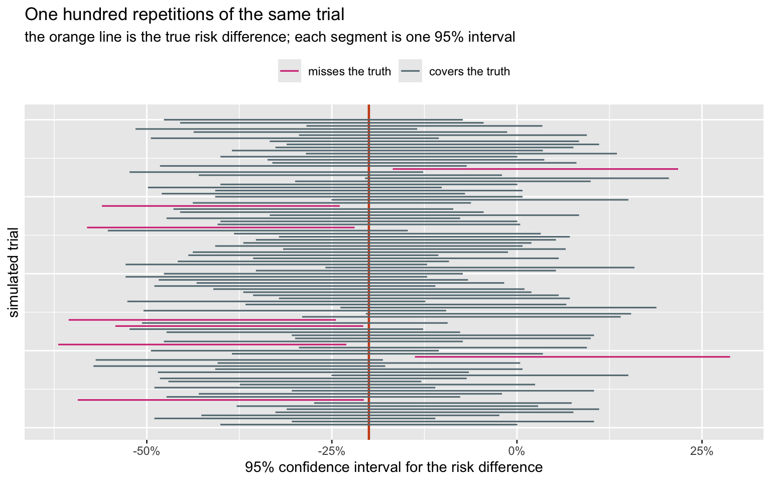
Two things to take from this. First, the guarantee is real but collective: some intervals miss, and nothing marks which. Second, the actual coverage here is 94.0%, not 95% – the Wald interval for a difference of proportions is known to undercover at this sample size. The nominal level is a promise about an idealisation.
The likelihood answer
The likelihoodist refuses to simulate hypothetical trials. The evidence is the likelihood function, and only the observed data enter it.
For a risk difference \(\Delta = p_t - p_c\) the baseline risk \(p_c\) is a nuisance parameter, so we profile it out: for each candidate \(\Delta\), maximise over \(p_c\).
loglik <- function(pc, delta) {
  pt <- pc + delta
  bad <- pc <= 0 | pc >= 1 | pt <= 0 | pt >= 1
  if (bad) return(-Inf)
  yc*log(pc) + (nc-yc)*log(1-pc) + yt*log(pt) + (nt-yt)*log(1-pt)
}

prof <- function(delta) {
  lo <- max(1e-9, -delta + 1e-9)
  hi <- min(1 - 1e-9, 1 - delta - 1e-9)
  optimize(function(pc) loglik(pc, delta), c(lo, hi), maximum = TRUE)$objective
}

grid_d  <- seq(-0.60, 0.15, by = 0.0005)
prof_ll <- vapply(grid_d, prof, numeric(1))
ll_max  <- max(prof_ll)

lik <- tibble(delta = grid_d,
              rel   = exp(prof_ll - ll_max))   # relative likelihood, max = 1
The relative likelihood rescales so the best-supported value is 1. A value with relative likelihood 1/8 is eight times less well supported by this data than the best one.
Support intervals
interval <- function(threshold) range(lik$delta[lik$rel >= threshold])

ints <- tibble(
  rule = c("1/8 support", "1/32 support", "95% likelihood ratio"),
  cut  = c(1/8, 1/32, exp(-qchisq(0.95, 1)/2))) |>
  rowwise() |>
  mutate(lo = interval(cut)[1], hi = interval(cut)[2]) |>
  ungroup()

ints |> mutate(across(c(cut, lo, hi), \(x) round(x, 4)))
## # A tibble: 3 × 4
## rule cut lo hi
## <chr> <dbl> <dbl> <dbl>
## 1 1/8 support 0.125 -0.426 -0.0115
## 2 1/32 support 0.0312 -0.482 0.052
## 3 95% likelihood ratio 0.146 -0.419 -0.02ggplot(lik, aes(delta, rel)) +
geom_area(fill = pal[["blue"]], alpha = 0.15) +
geom_line(colour = pal[["blue"]], linewidth = 1) +
geom_hline(data = ints, aes(yintercept = cut, linetype = rule),
colour = pal[["magenta"]], linewidth = 0.6) +
geom_vline(xintercept = 0, colour = pal[["orange"]],
linetype = "dotted", linewidth = 0.8) +
annotate("point", x = rd_hat, y = 1, colour = pal[["blue"]], size = 3) +
scale_x_continuous(labels = scales::percent) +
labs(title = "Profile relative likelihood for the risk difference",
subtitle = "the whole of the evidence, on one curve; dotted orange = no effect",
x = "risk difference", y = "relative likelihood",
linetype = NULL) +
theme(legend.position = "top")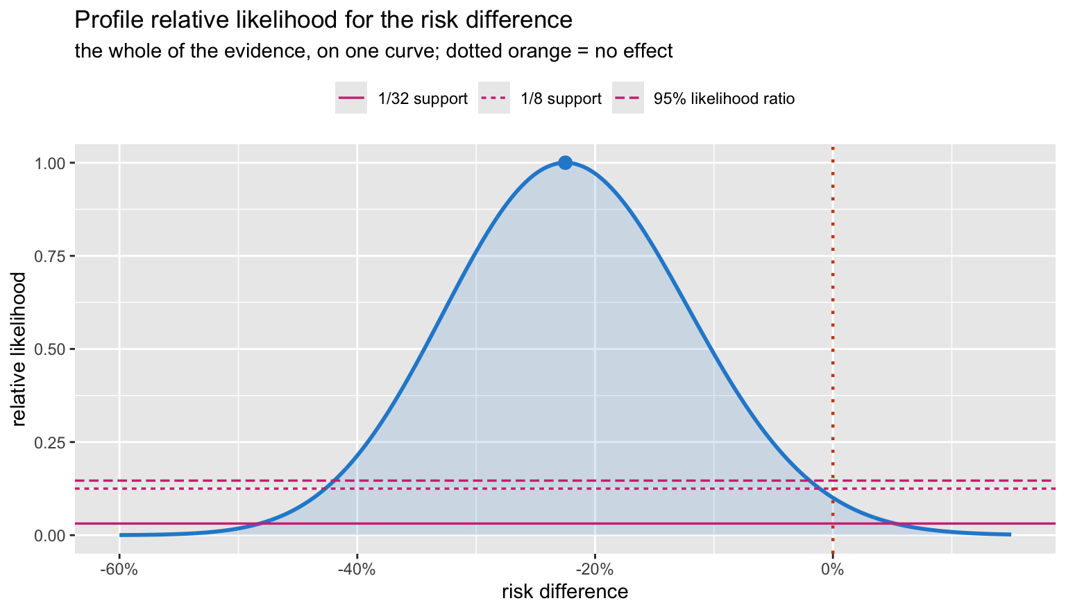
The curve peaks at the observed -22.5 points. “No effect” is not excluded by fiat, but it sits low on the curve: its relative likelihood is 0.101, so the data support the observed difference about 10 times more strongly than they support no difference at all.
Note the 95% likelihood-ratio interval (-0.419, -0.020) excludes
zero, while the Wald interval from prop.test – (-0.451,
0.001) – does not. Same data, two intervals, opposite verdicts at the
0.05 line.
What the likelihood deliberately does not give you is a probability. The curve is not a distribution over \(\Delta\): it does not integrate to one, and “relative likelihood 0.05” is not “5% probable”. To get a probability you must supply a prior, which is the next section and the whole of the disagreement.
The Bayesian answer
Put a prior on both arm rates, multiply by the likelihood, normalise. With two parameters we can do this exactly on a grid – no MCMC needed.
K  <- 400
gp <- (seq_len(K) - 0.5) / K

G <- expand.grid(pc = gp, pt = gp) |> as_tibble() |>
  mutate(loglik = yc*log(pc) + (nc-yc)*log(1-pc) +
                  yt*log(pt) + (nt-yt)*log(1-pt),
         rd  = pt - pc,
         lor = qlogis(pt) - qlogis(pc))

posterior <- function(logprior = 0) {
  lp <- G$loglik + logprior
  w  <- exp(lp - max(lp))
  w / sum(w)
}

w_flat <- posterior()                    # uniform Beta(1,1) on each arm
The joint posterior
ggplot(G, aes(pc, pt)) +
  geom_raster(aes(fill = w_flat)) +
  geom_abline(slope = 1, intercept = 0, colour = pal[["grey"]],
              linetype = "dashed", linewidth = 0.7) +
  annotate("point", x = pc_hat, y = pt_hat, colour = pal[["orange"]],
           shape = 4, size = 3.5, stroke = 1.4) +
  annotate("text", x = 0.225, y = 0.44, label = "high-flow worse",
           colour = pal[["grey"]], size = 3.6, hjust = 0) +
  annotate("text", x = 0.52, y = 0.085, label = "high-flow better",
           colour = pal[["grey"]], size = 3.6, hjust = 0) +
  scale_fill_gradient(low = "white", high = pal[["blue"]], guide = "none") +
  scale_x_continuous(labels = scales::percent) +
  scale_y_continuous(labels = scales::percent) +
  coord_equal(xlim = c(0.20, 0.72), ylim = c(0.05, 0.48)) +
  labs(title = "Joint posterior over the two arm risks",
       subtitle = "the dashed diagonal is 'no difference'; x marks the observed proportions",
       x = "risk, standard cannula", y = "risk, high-flow")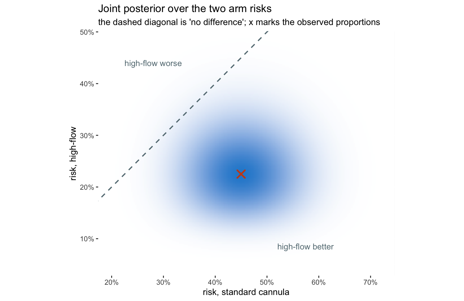
This picture makes the Bayesian answer almost tautological. The probability that high-flow is better is simply the share of posterior mass lying below the diagonal.
cri <- function(w, probs = c(0.025, 0.975)) {
  o  <- order(G$rd)
  cw <- cumsum(w[o])
  G$rd[o][vapply(probs, \(q) which.min(abs(cw - q)), integer(1))]
}

c(posterior_mean_RD = sum(w_flat * G$rd),
  CrI_lo = cri(w_flat)[1], CrI_hi = cri(w_flat)[2],
  P_benefit        = sum(w_flat[G$rd < 0]),
  P_benefit_gt_10pt = sum(w_flat[G$rd < -0.10]))
## posterior_mean_RD CrI_lo CrI_hi P_benefit
## -0.2142857 -0.4050000 -0.0150000 0.9818907
## P_benefit_gt_10pt
## 0.8717230A 98.2% probability that high-flow reduces desaturation, and a 87% probability that it does so by more than ten percentage points. These are answers to the clinical question. No frequentist quantity in this post is a probability about the treatment.
How much does the prior matter?
The honest objection to all this is that someone chose the prior. So show the range.
priors <- list(
  "uniform Beta(1,1)" = 0,
  "Jeffreys Beta(.5,.5)" = dbeta(G$pc, .5, .5, log = TRUE) +
                           dbeta(G$pt, .5, .5, log = TRUE),
  "skeptical: logOR ~ N(0, 0.5)"    = dnorm(G$lor,  0.0, 0.5, log = TRUE),
  "enthusiastic: logOR ~ N(-1, 0.5)" = dnorm(G$lor, -1.0, 0.5, log = TRUE))

ws <- lapply(priors, posterior)

tibble(prior = names(priors),
       mean_RD   = vapply(ws, \(w) sum(w * G$rd), numeric(1)),
       CrI_lo    = vapply(ws, \(w) cri(w)[1], numeric(1)),
       CrI_hi    = vapply(ws, \(w) cri(w)[2], numeric(1)),
       P_benefit = vapply(ws, \(w) sum(w[G$rd < 0]), numeric(1))) |>
  mutate(across(where(is.numeric), \(x) round(x, 3)))
## # A tibble: 4 × 5
## prior mean_RD CrI_lo CrI_hi P_benefit
## <chr> <dbl> <dbl> <dbl> <dbl>
## 1 uniform Beta(1,1) -0.214 -0.405 -0.015 0.982
## 2 Jeffreys Beta(.5,.5) -0.22 -0.412 -0.02 0.983
## 3 skeptical: logOR ~ N(0, 0.5) -0.115 -0.26 0.032 0.935
## 4 enthusiastic: logOR ~ N(-1, 0.5) -0.215 -0.358 -0.07 0.998# Every attainable rd is exactly (it - ic)/K, so bin on that integer
# difference. Running cut() on the floating-point values drops some of them
# exactly on a break, which aliases and leaves spurious notches in the curve.
marginal_rd <- function(w, step = 4) {
j <- as.integer(round(G$rd * K))
s <- tapply(w, j %/% step, sum)
bw <- step / K
tibble(rd = (as.integer(names(s)) + 0.5) * bw, dens = as.numeric(s) / bw)
}
marg <- bind_rows(lapply(names(ws), \(nm) mutate(marginal_rd(ws[[nm]]), prior = nm))) |>
mutate(prior = factor(prior, levels = names(priors)))
ggplot(marg, aes(rd, dens, colour = prior)) +
geom_vline(xintercept = 0, colour = pal[["grey"]], linetype = "dotted") +
geom_line(linewidth = 0.9) +
scale_colour_manual(values = unname(pal[c("blue", "cyan", "magenta", "green")])) +
scale_x_continuous(labels = scales::percent) +
coord_cartesian(xlim = c(-0.55, 0.2)) +
labs(title = "Posterior for the risk difference under four priors",
subtitle = "the skeptical prior pulls the estimate toward zero; it does not abolish it",
x = "risk difference", y = "posterior density", colour = NULL) +
theme(legend.position = "top")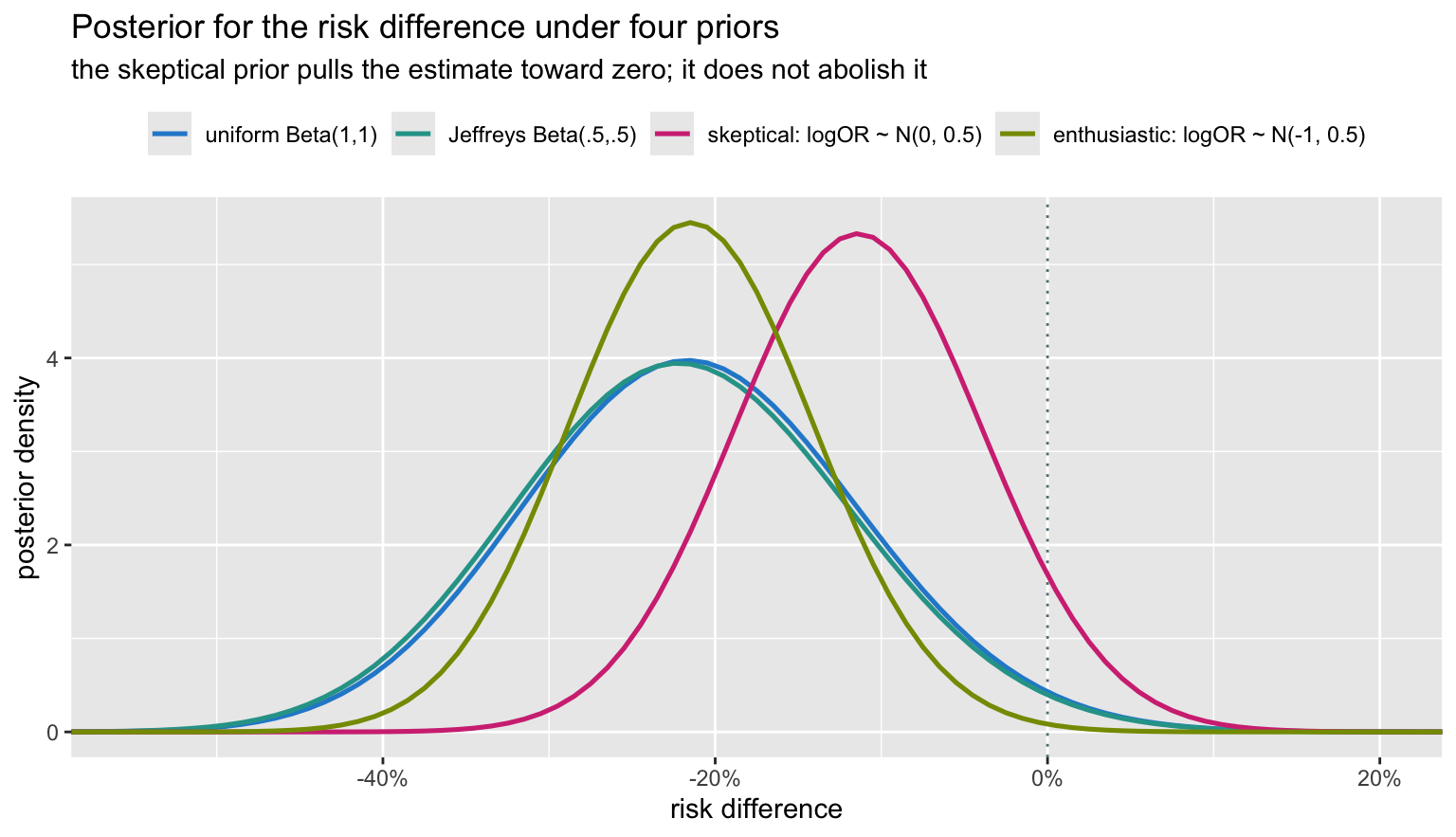
The skeptical prior – which says, before seeing anything, that large odds ratios are implausible – halves the estimated effect and moves P(benefit) from 0.982 down to 0.935. That is a real shift, and it is the right kind of argument to be having: it is about what we believed about bronchoscopy before the trial, stated out loud and quantified, rather than smuggled in through a choice of test.
Where they genuinely disagree
So far the three have mostly agreed. Here is a case where they cannot.
A respiratory ward audits its overnight desaturation alarms, asking whether genuine alarms are a minority – is the true rate below one half? Two registrars run the audit:
- Alice decides in advance to review 20 consecutive alarms. Six are genuine.
- Bob decides in advance to review alarms until he has found 6 genuine ones. The sixth arrives on the twentieth alarm.
Identical data: 6 genuine out of 20. Different sampling plans.
p0 <- 0.5
# Alice: binomial, n fixed at 20. P(6 or fewer genuine)
p_alice <- pbinom(6, 20, p0)
# Bob: negative binomial, 6 successes fixed. P(20 or more alarms needed)
#      = P(14 or more failures before the 6th success)
p_bob   <- 1 - pnbinom(13, 6, p0)

c(Alice = p_alice, Bob = p_bob)
## Alice Bob
## 0.05765915 0.03178406sd_a <- tibble(x = 0:20, prob = dbinom(0:20, 20, p0),
tail = x <= 6, plan = "Alice: fixed n = 20\n(binomial)")
sd_b <- tibble(x = 6:45, prob = dnbinom((6:45) - 6, 6, p0),
tail = x >= 20, plan = "Bob: stop at 6th genuine\n(negative binomial)")
bind_rows(sd_a, sd_b) |>
ggplot(aes(x, prob, fill = tail)) +
geom_col(width = 0.75) +
facet_wrap(~ plan, scales = "free") +
scale_fill_manual(values = unname(pal[c("grey", "orange")]), guide = "none") +
labs(title = "Same data, same null hypothesis, two sampling plans",
subtitle = sprintf("Alice's p = %.4f; Bob's p = %.4f. One crosses 0.05, the other does not.",
p_alice, p_bob),
x = "outcome of the audit", y = "probability under p = 0.5")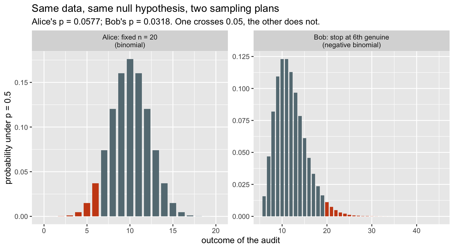
Alice reports 0.0577 and concludes nothing. Bob reports 0.0318 and declares genuine alarms a significant minority. Neither has made an error.
The p-value depends on the sampling plan because it is a tail area, and the tail is made of outcomes that could have occurred – and what could have occurred depends on when you intended to stop. Bob’s “more extreme” outcomes include audits of 30 and 40 alarms, which were never possible for Alice.
The likelihood does not care:
pg <- seq(0.05, 0.95, length.out = 400)

lik_alice <- dbinom(6, 20, pg)        # choose(20,6) * p^6 (1-p)^14
lik_bob   <- dnbinom(14, 6, pg)       # choose(19,5) * p^6 (1-p)^14

# the two differ only by a constant that does not involve p
list(ratio_is_constant = sd(lik_alice / lik_bob) < 1e-12,
     constant          = (lik_alice / lik_bob)[1])
## $ratio_is_constant
## [1] TRUE
##
## $constant
## [1] 3.333333tibble(p = rep(pg, 2),
rel = c(lik_alice / max(lik_alice), lik_bob / max(lik_bob)),
who = rep(c("Alice (binomial)", "Bob (negative binomial)"), each = length(pg))) |>
ggplot(aes(p, rel, colour = who, linetype = who)) +
geom_line(linewidth = 1.1) +
geom_vline(xintercept = 0.5, colour = pal[["orange"]], linetype = "dotted") +
scale_colour_manual(values = unname(pal[c("blue", "magenta")])) +
scale_linetype_manual(values = c("solid", "longdash")) +
labs(title = "The two likelihood functions are the same curve",
subtitle = "they differ by a constant factor, which cancels out of every comparison",
x = "true proportion of genuine alarms", y = "relative likelihood",
colour = NULL, linetype = NULL) +
theme(legend.position = "top")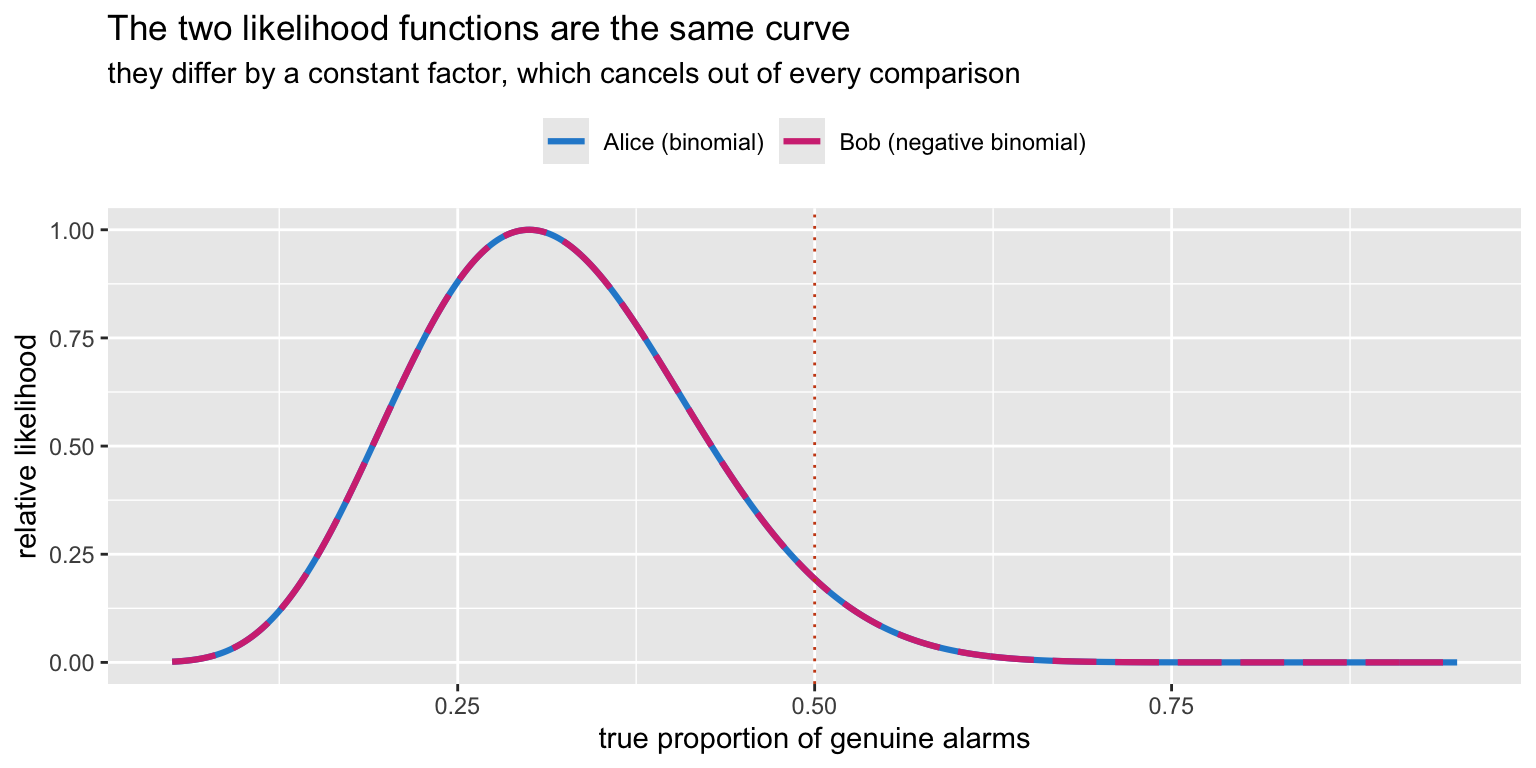
The dashed curve lies exactly on the solid one. Because the likelihoods are proportional, every likelihood ratio is identical, and so is every Bayesian posterior from a given prior. Alice and Bob reach the same conclusion.
This is the likelihood principle: the evidence in the data about the parameter is contained in the likelihood function. Frequentist inference violates it. Whether that is a fatal flaw or a reasonable price for procedural guarantees is the oldest argument in statistics, and it is a real argument – the frequentist is buying something with that violation, namely error control over repeated use, which matters enormously when the procedure is a regulatory standard applied thousands of times.
The bootstrap
The bootstrap is frequentist in logic – it approximates the sampling distribution – but it needs no formula and no normality assumption, which is why Harrell reaches for it so often. Resample patients within each arm, with replacement, and recompute.
ctrl <- c(rep(1, yc), rep(0, nc - yc))
trt  <- c(rep(1, yt), rep(0, nt - yt))

bd <- tibble(arm = factor(rep(c("standard", "high-flow"), c(nc, nt)),
                          levels = c("standard", "high-flow")),
             y   = c(ctrl, trt))

rd_stat <- function(data, i) {
  s <- data[i, ]
  mean(s$y[s$arm == "high-flow"]) - mean(s$y[s$arm == "standard"])
}

set.seed(42)
B  <- 4000
# strata = arm holds each resample to 40 patients per arm, as the design did
bo <- boot(bd, rd_stat, R = B, strata = bd$arm)
bc <- boot.ci(bo, type = c("perc", "bca", "basic"))

reps    <- as.vector(bo$t)
boot_ci <- rbind(percentile = bc$percent[4:5],
                 bca        = bc$bca[4:5],
                 basic      = bc$basic[4:5])
colnames(boot_ci) <- c("lo", "hi")

round(boot_ci, 4)
## lo hi
## percentile -0.425 -0.025
## bca -0.400 0.025
## basic -0.425 -0.025rms offers bootBCa() as a convenience
wrapper, but it hands boot.ci a placeholder statistic, so
the acceleration constant is estimated from an ambient random sample
rather than a proper jackknife. On a statistic this discrete that is
enough to move the interval between adjacent attainable values from one
run to the next. Calling boot directly, with the real
statistic, makes the BCa interval reproducible.
ggplot(tibble(rd = reps), aes(rd)) +
  geom_histogram(binwidth = 0.025, fill = pal[["blue"]],
                 colour = "white", alpha = 0.85) +
  geom_vline(xintercept = rd_hat, colour = pal[["blue"]], linewidth = 0.9) +
  geom_vline(xintercept = 0, colour = pal[["orange"]],
             linetype = "dotted", linewidth = 0.8) +
  geom_vline(xintercept = boot_ci["percentile", ], colour = pal[["magenta"]],
             linetype = "dashed", linewidth = 0.7) +
  scale_x_continuous(labels = scales::percent) +
  labs(title = "Bootstrap distribution of the risk difference",
       subtitle = sprintf("%d resamples; dashed = percentile interval, dotted orange = no effect", B),
       x = "risk difference", y = "resamples")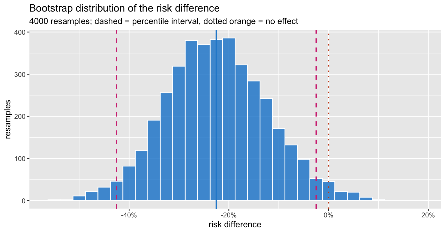
Two honest wrinkles. The percentile interval (-0.425, -0.025) excludes zero; the bias-corrected and accelerated interval (-0.400, 0.025) reaches it. BCa adjusts for bias and skewness in the bootstrap distribution, is generally the better interval, and is the more conservative one here – it alone among the bootstrap methods declines to exclude no effect.
And with 40 patients per arm the risk difference can only take 150 distinct values in any resample, so the bootstrap distribution is genuinely lumpy. The histogram is honest about that; a kernel density curve would have sold you a smoothness the data do not have.
The same machinery works on a fitted model. rms::bootcov
refits the model on each resample and returns a bootstrap covariance
matrix:
d <- tibble(arm = factor(rep(c("standard", "high-flow"), c(nc, nt)),
                         levels = c("standard", "high-flow")),
            desat = c(ctrl, trt))

dd <- datadist(d)
assign("dd", dd, envir = globalenv())      # rms looks this up by name
options(datadist = "dd")

f  <- lrm(desat ~ arm, data = d, x = TRUE, y = TRUE)
set.seed(7)
bf <- bootcov(f, B = 1000)

c(log_OR          = coef(f)[2],
  model_SE        = sqrt(diag(vcov(f)))[2],
  bootstrap_SE    = sqrt(diag(vcov(bf)))[2],
  boot_pct_lo     = quantile(bf$boot.Coef[, 2], 0.025, na.rm = TRUE),
  boot_pct_hi     = quantile(bf$boot.Coef[, 2], 0.975, na.rm = TRUE)) |> round(4)
## log_OR.arm=high-flow model_SE.arm=high-flow
## -1.0361 0.4943
## bootstrap_SE.arm=high-flow boot_pct_lo.2.5%
## 0.5187 -2.1849
## boot_pct_hi.97.5%
## -0.1331All three on one axis
Now put the likelihood curve, the bootstrap distribution and the posterior on the same plot. They are different objects – a relative likelihood, a sampling distribution and a probability distribution over the parameter – so each is normalised to unit area purely so the shapes can be compared.
norm_area <- function(x, y) y / sum(y * c(diff(x), 0)[seq_along(y)])

lik_n  <- lik |> filter(delta >= -0.6, delta <= 0.2) |>
  mutate(dens = norm_area(delta, rel), curve = "likelihood (normalised)")

post_n <- marginal_rd(w_flat, step = 2) |>
  transmute(delta = rd, dens, curve = "posterior (flat prior)")

bden   <- density(reps, adjust = 1.3)
boot_n <- tibble(delta = bden$x, dens = bden$y, curve = "bootstrap distribution")

ggplot(bind_rows(lik_n, post_n, boot_n),
       aes(delta, dens, colour = curve, linetype = curve)) +
  geom_vline(xintercept = 0, colour = pal[["grey"]], linetype = "dotted") +
  geom_line(linewidth = 1) +
  scale_colour_manual(values = unname(pal[c("blue", "magenta", "green")])) +
  scale_linetype_manual(values = c("solid", "longdash", "dotdash")) +
  scale_x_continuous(labels = scales::percent) +
  coord_cartesian(xlim = c(-0.55, 0.15)) +
  labs(title = "Three traditions, one small trial",
       subtitle = "different philosophies, nearly the same curve",
       x = "risk difference", y = "density (each normalised to unit area)",
       colour = NULL, linetype = NULL) +
  theme(legend.position = "top")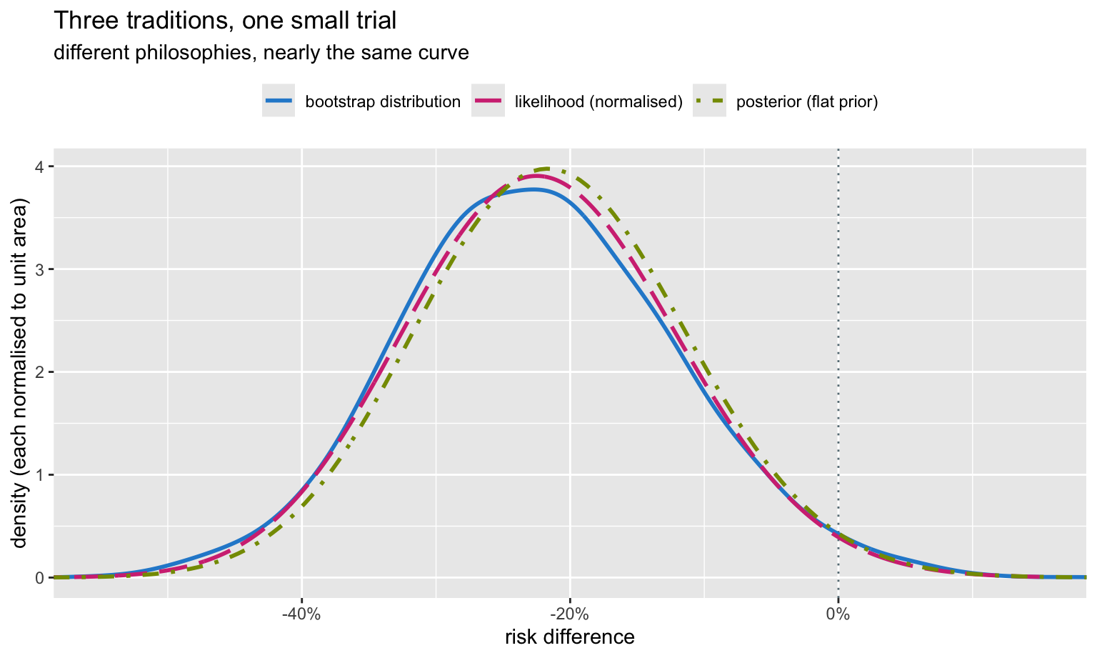
They very nearly coincide. This is not a coincidence and it is not a proof of equivalence: with a flat prior the posterior is proportional to the likelihood, and the bootstrap distribution is a nonparametric estimate of the sampling distribution, which in regular problems has the same width. Compare:
c(bootstrap_P_harm = mean(reps >= 0),
  posterior_P_harm = sum(w_flat[G$rd >= 0]))
## bootstrap_P_harm posterior_P_harm
## 0.02275000 0.01810934The bootstrap proportion above zero (0.023) and the posterior probability of no benefit (0.018) both land near 2%, although one is a statement about resampled datasets and the other a statement about the parameter. They are close, not equal, and the residual gap is real. This numerical near-equivalence is why the bootstrap so often feels Bayesian, and why Harrell treats it as a practical bridge. It is a regularity of well-behaved problems, not a theorem: it degrades with strong priors, small counts, boundaries and heavy nuisance-parameter structure.
Everything that disagreed, in one picture
pt_ci <- prop.test(c(yt, yc), c(nt, nc))$conf.int

res <- tribble(
  ~paradigm,      ~method,                         ~lo,                 ~hi,
  "frequentist",  "Wald interval (prop.test)",     pt_ci[1],            pt_ci[2],
  "frequentist",  "bootstrap percentile",          boot_ci["percentile","lo"], boot_ci["percentile","hi"],
  "frequentist",  "bootstrap BCa",                 boot_ci["bca","lo"], boot_ci["bca","hi"],
  "likelihood",   "95% likelihood ratio",          ints$lo[3],          ints$hi[3],
  "likelihood",   "1/8 support",                   ints$lo[1],          ints$hi[1],
  "likelihood",   "1/32 support",                  ints$lo[2],          ints$hi[2],
  "Bayesian",     "95% CrI, uniform prior",        cri(ws[[1]])[1],     cri(ws[[1]])[2],
  "Bayesian",     "95% CrI, Jeffreys prior",       cri(ws[[2]])[1],     cri(ws[[2]])[2],
  "Bayesian",     "95% CrI, skeptical prior",      cri(ws[[3]])[1],     cri(ws[[3]])[2],
  "Bayesian",     "95% CrI, enthusiastic prior",   cri(ws[[4]])[1],     cri(ws[[4]])[2]) |>
  mutate(paradigm = factor(paradigm, levels = c("frequentist", "likelihood", "Bayesian")),
         method   = factor(method, levels = rev(method)),
         excludes = hi < 0)

ggplot(res, aes(y = method)) +
  geom_vline(xintercept = 0, colour = pal[["orange"]], linewidth = 0.8) +
  geom_segment(aes(x = lo, xend = hi, yend = method, colour = paradigm),
               linewidth = 1.1) +
  geom_point(aes(x = rd_hat), colour = pal[["grey"]], size = 1.8) +
  geom_point(aes(x = lo, colour = paradigm), size = 2) +
  geom_point(aes(x = hi, colour = paradigm), size = 2) +
  facet_grid(paradigm ~ ., scales = "free_y", space = "free_y", switch = "y") +
  scale_colour_manual(values = unname(pal[c("blue", "magenta", "green")]),
                      guide = "none") +
  scale_x_continuous(labels = scales::percent) +
  labs(title = "Ten intervals for one risk difference",
       subtitle = "orange line = no effect. Whether the trial is 'positive' depends on the row you read.",
       x = "risk difference", y = NULL) +
  theme(strip.placement = "outside")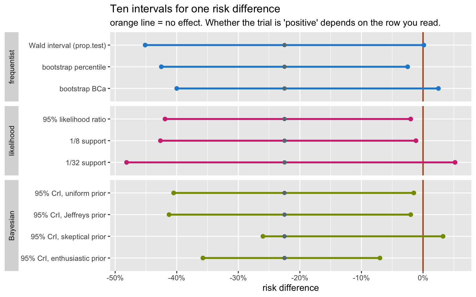
res |>
  transmute(paradigm, method,
            interval = sprintf("(%6.3f, %6.3f)", lo, hi),
            `excludes 0` = ifelse(excludes, "yes", "no")) |>
  as.data.frame()
## paradigm method interval excludes 0
## 1 frequentist Wald interval (prop.test) (-0.451, 0.001) no
## 2 frequentist bootstrap percentile (-0.425, -0.025) yes
## 3 frequentist bootstrap BCa (-0.400, 0.025) no
## 4 likelihood 95% likelihood ratio (-0.419, -0.020) yes
## 5 likelihood 1/8 support (-0.426, -0.011) yes
## 6 likelihood 1/32 support (-0.481, 0.052) no
## 7 Bayesian 95% CrI, uniform prior (-0.405, -0.015) yes
## 8 Bayesian 95% CrI, Jeffreys prior (-0.412, -0.020) yes
## 9 Bayesian 95% CrI, skeptical prior (-0.260, 0.032) no
## 10 Bayesian 95% CrI, enthusiastic prior (-0.357, -0.070) yes6 of the 10 intervals exclude zero. A reader told only “p = 0.058, not significant” would have no idea that this was the situation.
What to actually do
The practical position, and it is largely Harrell’s:
Stop reporting significance. The dichotomy at 0.05 is where almost all the damage happens. In this trial it is the single thing that varies most between defensible analyses. Report the estimate and an interval.
Report the effect with its uncertainty, on a clinical scale. A risk difference of -22.5 points with an interval reaching from roughly 42 points of benefit to roughly zero is a complete, honest summary. Nothing is added by a verdict.
Use the bootstrap when the formula is doubtful. It
costs nothing, assumes little, and rms has it built in for
fitted models. Prefer BCa.
Say what you believed beforehand. A Bayesian analysis with a pre-specified skeptical prior is the most honest version of a small trial, because the skepticism is written down and quantified rather than applied informally at the end by a reader who is unimpressed.
Report posterior probabilities when the audience must act. “A 98% probability of benefit, 87% probability of benefit exceeding 10 points” is directly usable by someone deciding whether to buy the equipment. “p = 0.058” is not.
And the meta-point: in this trial the three traditions produced nearly the same curve. The disagreement was never really between frequentism and Bayes. It was between any reasonable analysis and the practice of collapsing it to a yes/no at 0.05.
References
- Harrell FE. Biostatistics for Biomedical Research, hbiostat.org. Chapters on probability, hypothesis testing and the bootstrap.
- Harrell FE. Regression Modeling Strategies, 2nd ed. Springer, 2015.
- Lindley DV, Phillips LD. Inference for a Bernoulli process (a Bayesian view). Am Stat 1976;30:112–119.
- Berger JO, Wolpert RL. The Likelihood Principle, 2nd ed. IMS, 1988.
- Royall R. Statistical Evidence: A Likelihood Paradigm. Chapman & Hall, 1997.
- Spiegelhalter DJ, Freedman LS, Parmar MKB. Bayesian approaches to randomized trials. J R Stat Soc A 1994;157:357–416.
- Greenland S, et al. Statistical tests, P values, confidence intervals, and power: a guide to misinterpretations. Eur J Epidemiol 2016;31:337–350.
- Efron B, Tibshirani RJ. An Introduction to the Bootstrap. Chapman & Hall, 1993.